Week 7 - Simulation of a 1D Super-sonic nozzle flow simulation using Macormack Method
Simulation of a 1D Super-sonic nozzle flow simulation using Macormack Method
The main idea for understanding conservative and Non- conservative form of g.e equation is based on the understanding of control volume status.
Reynold's Transport Theorem :
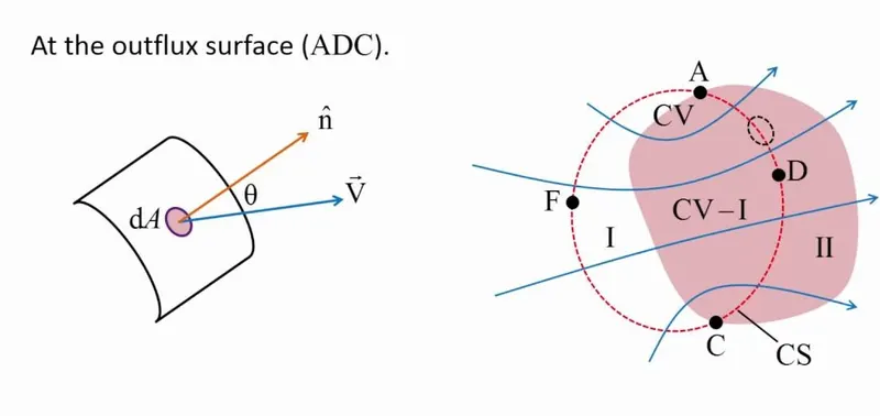
The basic idea that goes into understanding control volume approach is derived from Reynolds Transport theorem, which clearly depicts that mass outside the control surface of a control volume directed by the flux vector is the sum of rate of change of mass inside the system + rate of mass entering inside the system.
`frac{dN}{dT}|_(s y s t e m) = frac{del}{delt}int_(C V )( rho*n*dV) + int_(C S) rho*n*(vec V_ r*n)*dA`
RTT is a very strong theorem, any g.e could be derived from this theorem and idea. If we carefully observe the equation, RTT tells us that rate of mass moving outside the control surface of the control volume is dependant on the relative velocity of the control volumme w.r.to the medium in which it is present.
Special Cases :
- If the fluid is moving and the control volume is at rest, then
`vec V_r = vecV` which is called as the Stationary Control Volume
- If the fluid is moving and the control volume is also moving, but the volume of the control volume is Non-Deformable
`vec V_r ne vecV`
- If the fluid is moving and the control volume is also moving, but the volume of the control volume is Deformable
`vec V_r ne vecV`
NOTE : Assuming a Deformable control volume for this case
CASE I : Finite Control Volume fixed in Space
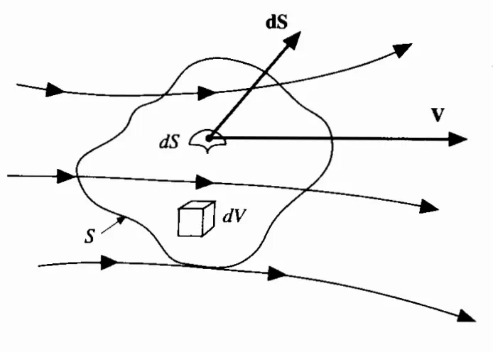
The fluid moves through the fixed control volume, flowing across the control surface. At a point on the control surface the flow velocity is V and the vector elemental surface area is dS, Also let dV be an elemental volume inside the finite control volume. Applied to this control volume, our fundamental physical principle that mass is conserved means
Net mass flow out time rate of = decrease of mass through surface 'S' inside control volume `=> (star)`
Note that by convention, dS always points in a direction out of the control volume. Hence, when V also points out of the control volume
The product pV • dS is positive. Moreover, when V points out of the control volume, the mass flow is physically leaving the control volume; i.e., it is an ouif/ow. Hence, a positive p V · dS denotes an outflow. In turn, when V points into the control volume, pV • dS is negative. Moreover, when V points inward, the mass flow is physically entering the control volume; i.e., it is an inflow. Hence, a negative p V · dS denotes an inflow. The net mass flow out of the entire control volume through the control surface S is the summation over S of the elemental mass flow
In the limit, this becomes a surface integral, which is
`B = intint_S rho*V*ds`
The mass contained within the elemental volume di/" is p di/". The total mass inside the control volume is
`intintint_V (rho)*dV`
The time rate of increase of mass inside V is then
`-frac{del}{delt}* intintint_V (rho)*dV`
Therefore from equation `star`:
`frac{del}{delt}* intintint_V (rho)*dV` +`intint_S rho*V*ds = 0` `=> (1)`
Equation (1) is Integral form of Continuity Equation which is called the CONSERVATIVE FORM of the Continuity Equation
CASE II : Finite Control Volume moving with Fluid
Control volume, as it moves with the fluid, is always composed of the same identifiable elements of mass; i.e., the moving
control volume has a fixed mass.
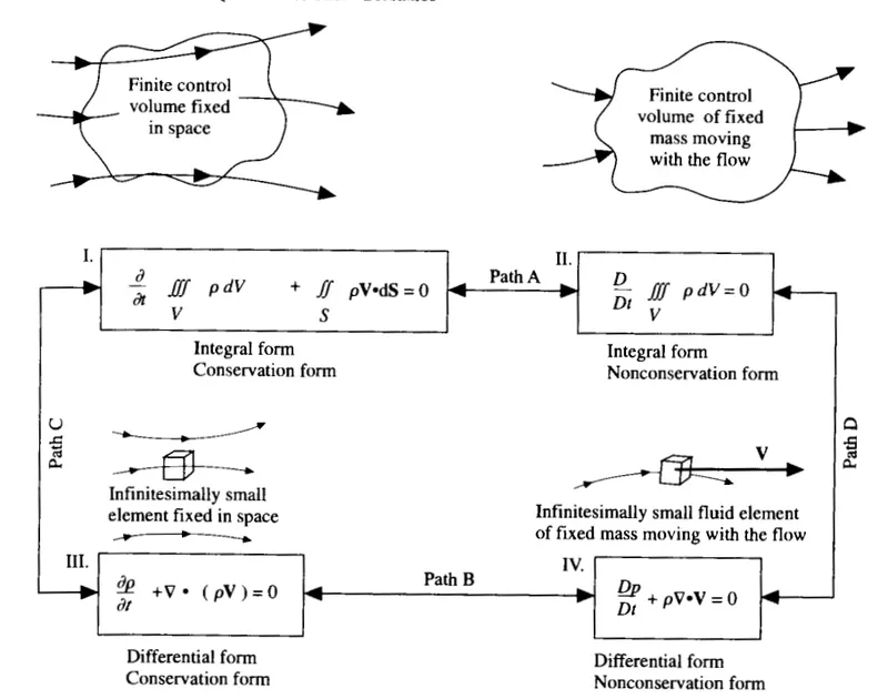
On the other hand, as this fixed mass moves downstream, the shape and volume of the finite control volume can in general change.
Consider an infinitesimally small element of volume dV inside this finite control volume; the mass of this small element is `rho*dV`, where`rho` is the local density.
Then, the total mass of the finite control volume is given by
`Mass = intintint_V (rho)*dV`
The volume integral is taken over the whole moving control volume V. However, V is changing as the control volume moves downstream. On the other hand, the physical principle that mass is conserved, when applied to this model of the flow, simply states that the mass is constant as the control volume moves with the flow.
Since this finite control volume is made up of an infinite number of infinitesimally small fluid elements, all with a fixed, unchanging mass, and hence all with substantial denvatives of these unchanging masses equal to zero, we can write for the finite control volume as below
`frac{D}{Dt}intintint_V (rho)*dV = 0` `=> (2)`
Equation (2) is Integral form of Continuity Equation which is called the NON-CONSERVATIVE FORM of the Continuity Equation
Converting Integral form of the Continuity equations to PDE
Let dx be the C/S of the nozzle
Let `rho`,V, P, e be the density, velocity, pressure & internal energy of the medium entering the nozzle inlet at the start of dx.
By using Taylor's Series expansion :
We can find out the values of these parameters for increase in 'dx' amount of its domain length
`frac{del}{delt}* intintint_V (rho)*dV` +`intint_S rho*V*ds = 0` `=> (1)`
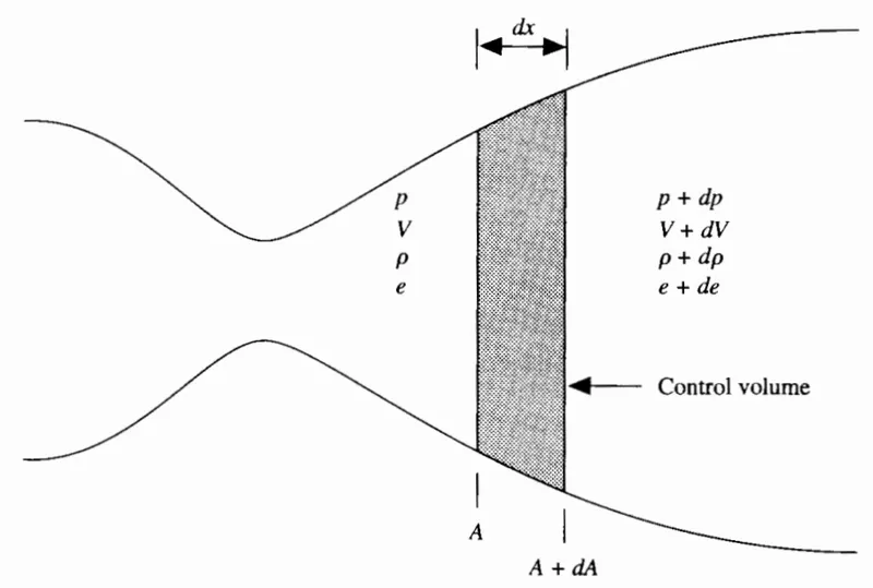
Mass flow rate from the left end of the control volume is `rho*V*A`
Mass flow rate from the right end of the control volume is as follows
`(rhoV + rhodV +drhoV + drhodV)*(A+dA)`
Mass Inlet = `-rho*V*A`
Mass Outlet = `(rhoV + rhodV +drhoV + drhodV)*(A+dA)`
`:.`Net rate of increase of mass = `-d(rhoAV)`
`:.``d(rhoAV)` =`intint_S rho*V*ds`
Discretization Techniques :
Maccormack's Technique
Maccormack method is also an explicit finite-difference technique which is second-order-accurate in both space and time. It consists of two-step, First the Predictor Step & then the Corrector Step.
Let us consider a variable f(x) which can be any flow variable such as velocity, pressure, density, temperature, etc.
1. Initialising the profile of of flow variables
2. Predictor Step - Calculating the time derivative by forward differencing the space derivatives
`(frac{delf}{delt})_p = frac{f(i+1)_(i n i t i a l) -f(i)_(i nitial)}{Deltax}`
3. Solution Update for the predictor step
`f_p = f_( i nitial) + (frac{delf}{delt})_p*Deltat`
4. Corrector Step - Predictor step values of 'f' are rearward differenced to calculate time derivatives
`(frac{delf}{delt})_C = frac{f(i)_(p) -f(i-1)_p}{Deltax}`
5. Averaging time derivatives
`(frac{delf}{delt})_(avg) = 0.5*[(frac{delf}{delt})_(p) + (frac{delf}{delt})_(c) ]`
6. Final solution update
Implementing average time derivatives for calculation
`(f_i)^(n+1) = (f_(i n itial))^(n) + (frac{delf}{delt})_(avg)*Deltat`
Boundary Condition :
Grid points 1 and N represent the two boundary points on the x axis. Point 1 is essentially in the reservoir. It represents
an inflow boundary, with flow coming from the reservoir and entering the nozzle.
In contrast, point N is an outflow boundary, with flow leaving the nozzle at the nozzle exit.
Moreover, the flow velocity at point 1 is a very low, subsonic value. (The flow velocity at point 1, which corresponds to a finite area ratio `A_1/A^(star)`, cannot be precisely zero; if it were, there would be no mass flow entenng the nozzle. Hence, point 1 does not correspond exactly to the reservoir.
Unsteady, inviscid flow is governed by equations, and therefore for one-dimensional unsteady flow is governed by hyperbolic characteristic lines through any point in xt plane
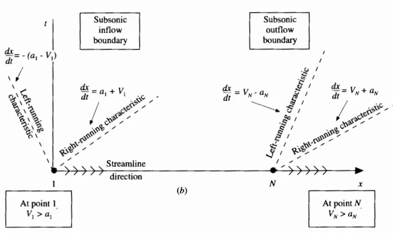
Subsonic inflow boundary (point 1):
Here, we must allow one variable to float; we choose the velocity V1, because on a physical basis we know the mass flow through the nozzle must be allowed to adJust to the proper steady state and allowing V1 to float makes the most sense as part of this adjustment.
The value of V1 changes with time and is calculated from information provided by the flow-field solution over the internal points. We use linear extrapolation from points 2 and 3 to calculate V1. The slope of the linear extrapolation hne 1s determined from points 2 and 3 as
Slope = `frac{V_3 - V_2}{Deltax}`
Using this slope to find V1 by linear extrapolation, we have
`V_1 = [V_2 - frac{V_3 - V_2}{Deltax}*Deltax]`
All other flow-field variables are specified. Since point 1 is viewed as essentially the reservoir, we stipulate the density and temperature at point 1 to be their respective stagnation values, `rho_0`and To, respectively.
Supersonic outflow boundary (point N)
Here, we must allow all flow-field variables to float We again choose to use lmear extrapolation based on the flowfield values at the internal points, Specifically, we have, for the nondimensional variables,
VN = 2VN-1 - VN-2
PN = 2PN-1 - PN-2
TN= 2TN-I - TN-2
Application of Maccormacks Technique to Nozzle and Solving PDEs :
Non-dimensional Non-Conservative form of the Governing Equation :
1. Continuity Equation
`frac{delrho'}{delt'} = -[rho'*frac{delV'}{delx'}] - [rho'*V'*frac{dellnA'}{delx'}]-[V'*frac{delrho'}{delx'}]`
2. Momentum Equation
`frac{delV'}{delt' } = -V'*frac{delV'}{delx'} - 1/gamma*[frac{delT'}{delx'}+frac{T'}{rho'}*frac{delrho'}{delx'}]`
3. Energy Equation
`frac{delT'}{delt' } = -V'*frac{delT'}{delx'} - (gamma-1)*T'*[frac{delV'}{delx'}+V'*frac{dellnA'}{delx'}]`
Non-dimensional Conservative form of the Governing Equation :
1. Continuity Equation
`frac{del(rho'*A')}{delt'} + frac{del(rho'*A'*V')}{delx'} = 0`
2. Momentum Equation
`frac{del(rho'*A'*V')}{delt'} + frac{del[rho'A'(V')^2 + (1/gamma)P'A']}{delx'}= (1/gamma)P'frac{delA'}{delx'}`
3. Energy Equation
`frac{del[rho'*(frac{e'}{gamma -1} + (gamma/2)*(V')^2)*A']}{delt'} + frac{del[rho'*(frac{e'}{gamma -1} + (gamma/2)*(V')^2)V'A' + P'A'V']}{delx'} = 0`
MatLab Code (Conservative & Non-Conservative Form) :
%% Simulating Quasi 1-D Nozzle flow equation for Conservative form

% Defining the domain grid parameters

% No of grid points
n = 31;

% Total lengthof doamin with grid spacing
x = linspace(0,3,n);

% Grid spacing
dx = x(2)-x(1);

% Defining gamma

gamma = 1.4;

% No of times iteration to be performed
nt = 1400;

% Defining Courant number
C = 0.5;
%% Conservative Form

tic
% [discharge,mach_number,rho,v,T,pressure,discharge_thrt,mach_number_thrt,rho_thrt,v_thrt,T_thrt,pressure_thrt] = conservative_equation(x,dx,n,gamma,C,nt);
[discharge,mach_number,rho,v,T,pressure,discharge_thrt,mach_number_thrt,rho_thrt,v_thrt,T_thrt,pressure_thrt] = conservative_equation(x,dx,n,gamma,nt,C)
run_time_cons = toc;
sprintf('Run Time for Conservative form = %0.4f',run_time_cons);
hold on

% Plotting all critical parameters values for various values of Time steps
figure(5)
% Pressure vs Time steps
subplot(4,1,1)
plot(pressure_thrt,'color','r','linewidth',1.5)
xlabel('Timestep')
ylabel('Pressure of medium at Throat')
% axis([0 1400 1 1.5])
grid minor
title('Pressure variation for various time steps - Non Conservation form')

% Density vs Time steps
subplot(4,1,2)
plot(rho_thrt,'color','y','linewidth',1.5)
xlabel('Timestep')
ylabel('Density of medium at Throat')
% axis([0 1400 1 1.5])
grid minor
title('Density variation for various time steps - Non Conservation form')

% Temperature vs Time steps
subplot(4,1,3)
plot(T_thrt,'color','g','linewidth',1.5)
xlabel('Timestep')
ylabel('Temperature of medium at Throat')
% axis([0 1400 1 1.5])
grid minor
title('Temperature variation for various time steps - Non Conservation form')


% Mach-Number vs Time steps
subplot(4,1,4)
plot(mach_number_thrt,'color','k','linewidth',1.5)
xlabel('Timestep')
ylabel('Mach-Number of medium at Throat')
% axis([0 1400 0 1.5])
grid minor
title('Mach-number variation for various time steps - Non Conservation form')


%% Plotting steady state parameter values for various values of Time steps
figure(6)

% Pressure vs Time steps
subplot(4,1,1)
plot(pressure,'color','r','linewidth',1.5)
xlabel('Timestep')
ylabel('Pressure')
% axis([0 1400 1 1.5])
grid minor
title('Pressure variation for various time steps - Conservation form')

% Density vs Time steps
subplot(4,1,2)
plot(rho,'color','y','linewidth',1.5)
xlabel('Timestep')
ylabel('Density')
% axis([0 1400 1 1.5])
grid minor
title('Density variation for various time steps - Conservation form')

% Temperature vs Time steps
subplot(4,1,3)
plot(T,'color','g','linewidth',1.5)
xlabel('Timestep')
ylabel('Temperature')
% axis([0 1400 1 1.5])
grid minor
title('Temperature variation for various time steps - Conservation form')

% Mach-Number vs Time steps
subplot(4,1,4)
plot(mach_number,'color','k','linewidth',1.5)
xlabel('Timestep')
ylabel('Mach-Number of medium at Throat')
% axis([0 1400 0 1.5])
grid minor
title('Mach-number variation for various time steps - Conservation form')
Matlab function for Conservative Form :
function [discharge,mach_number,rho,v,T,pressure,discharge_thrt,mach_number_thrt,rho_thrt,v_thrt,T_thrt,pressure_thrt] = conservative_equation(x,dx,n,gamma,nt,C)

% Intiliasing density & Temperature profiles

          for l = 1:n
              if x(l) <= 0.5
                  rho(l) = 1;
                  T(l) = 1;

              elseif (x(l)> 0.5 && x(l) <= 1.5)
                  rho(l) = 1 - 0.366*(x(l) - 0.5);
                  T(l) = 1 - 0.167*(x(l) - 0.5);

              elseif (x(l) > 1.5 && x(l) <= 3)
                  rho(l) = 0.634 - 0.3879*(x(l) - 1.5);
                  T(l) = 0.833 - 0.3507*(x(l) - 1.5);
                  pressure(l) = rho(l)* T(l);
              end

              % Determining Velocity & Nozzle Area profile
              a(l) = 1 + 2.2*(x(l) - 1.5).^2;
              v(l) = (0.59)/(rho(l)*a(l));
              discharge(l) = rho(l).*a(l).*v(l);

          end

               % Initializing the values of Discharge & Throat
          discharge_initial1 = rho.*a.*v;
          throat = find(a==1);

           % Defining the Time step "dt"
           dt = min((C.*dx)./(sqrt(T) + v));


          % Defining the initial solution vector
          U1 = rho.*a;
          U2 = rho.*a.*v;
          U3 = rho.*a.*((T./(gamma-1))+((gamma/2).*v.^2));

          % Starting time loop counter
          sim_time = 0;

          % Initilaising Time loop counter i
          for i = 1:nt

              % Storing Copy of Initial Data
              U1_old = U1;
              U2_old = U2;
              U3_old = U3;


          % Calculating Initial flux vector
           F1 = U2;
           F2 = ((U2.^2)./U1)+((gamma - 1)/gamma)*(U3 - (gamma/2)*(U2.^2)./U1);
           F3 = ((gamma.*U2.*U3)./U1) - (gamma*(gamma-1)/2)*((U2.^3)./(U1.^2));

          % Predictor St;ep
          for k = 2:n-1

              % Source Term
              J(k) = (1/gamma)*rho(k)*T(k)*((a(k+1)-a(k))/dx);

              % Continuity Term
              dU1_dt_p(k) = -((F1(k+1)-F1(k))/dx);

              % Momentum Term
              dU2_dt_p(k) = -((F2(k+1)-F2(k))/dx)+ J(k);

              % Energy Term
              dU3_dt_p(k) = -((F3(k+1)-F3(k))/dx);

              % Updating Solution vector

              U1(k) = U1(k) + dU1_dt_p(k)*dt;
              U2(k) = U2(k) + dU2_dt_p(k)*dt;
              U3(k) = U3(k) + dU3_dt_p(k)*dt;

          end


          % Updating Flux vector

          F1 = U2;
          F2 = ((U2.^2)./U1) + ((gamma-1)/gamma)*(U3-(gamma/2)*(U2.^2)./U1);
          F3 = ((gamma.*U2.*U3)./U1)-(gamma*(gamma-1)/2)*((U2.^3)./(U1.^2));

          % Defining Primitive Variables

          rho = U1./a ;
          v = U2./U1;
          T = (gamma-1)*((U3./U1)-((gamma/2)*(v.^2)));
          pressure = rho.*T;

      % Corrector Step
        for j = 2:n-1

              % Source Term
              J(j) = (1/gamma)*rho(j)*T(j)*((a(j)-a(j-1))/dx);

              % Continuity Term
              dU1_dt_c(j) = -((F1(j)-F1(j-1))/dx);

              % Momentum Term
              dU2_dt_c(j) = -((F2(j)-F2(j-1))/dx)+ J(j);

              % Energy Term
              dU3_dt_c(j) = -((F3(j)-F3(j-1))/dx);

        end


            % Averaging time derivative
            dU1_dt = 0.5*(dU1_dt_p + dU1_dt_c);
            dU2_dt = 0.5*(dU2_dt_p + dU2_dt_c);
            dU3_dt = 0.5*(dU3_dt_p + dU3_dt_c);

            % Updated Solution Vector
       for  m = 2:n-1

            U1(m) = U1_old(m) + dU1_dt(m)*dt;
            U2(m) = U2_old(m) + dU2_dt(m)*dt;
            U3(m) = U3_old(m) + dU3_dt(m)*dt;

       end


      % Applying Boundary Conditions

      % Inlet Boundary Conditions
      U1(1) = rho(1)*a(1);
      U2(1) = 2*U2(2) - U2(3);
      v(1) = U2(1)./U1(1);
      U3(1) = U1(1)*((T(1)/(gamma-1))+((gamma/2)*(v(1)^2)));


      % Outlet Boundary Conditions
      U1(n) = 2*U1(n-1)-U1(n-2);
      U2(n) = 2*U2(n-1)-U2(n-2);
      U3(n) = 2*U3(n-1)-U3(n-2);

      % Calculating corrcted primitive non dimensional variable for next time step
      rho = U1./a;
      T = (gamma-1)*((U3./U1)-((gamma/2)*(v.^2)));
      pressure = rho.*T;
      discharge = rho.*a.*v;
      mach_number = (v./sqrt(T));

      % Non dimensional parameters (AT THROAT)
      rho_thrt(i) = rho(throat);
      v_thrt(i) = v(throat);
      T_thrt(i) = T(throat);
      pressure_thrt(i) = pressure(throat);
      discharge_thrt(i) = discharge(throat);
      mach_number_thrt(i) = mach_number(throat);

      sim_time = sim_time + 1;

      % Plotting

      % Non dimensional mass flow rate at diff time step
      figure(4)

   if i == 1
        plot(x,discharge_initial1,'--','color','k','LineWidth',1,'Displayname','0th Time step')
        hold on
   end

   if i == 10
        plot(x,discharge,'color','r','LineWidth',1,'Displayname','10th Time step')
        hold on

    elseif i == 50
        plot(x,discharge,'color','y','LineWidth',1,'Displayname','50th Time step')
        hold on

    elseif i == 100
        plot(x,discharge,'color','g','LineWidth',1,'Displayname','100th Time step')
        hold on

    elseif i == 150
        plot(x,discharge,'color','k','LineWidth',1,'Displayname','150th Time step')
        hold on

    elseif i == 200
        plot(x,discharge,'color','m','LineWidth',1,'Displayname','200th Time step')
        hold on

    elseif i== 400
        plot(x,discharge,'color','c','LineWidth',1,'Displayname','400th Time step')
        hold on
    elseif i== 800
        plot(x,discharge,'color','b','LineWidth',1,'Displayname','800th Time step')
        hold on


    end


  title('Discharge distribution across Nozzle domain for various time steps-Conservation form');
  grid minor
  legend('0th Time step','10th Time step','50th Time step','100th Time step','150th Time step','200th Time step','400th Time step','800th Time step')
  xlabel('Nozzle Domain (length)');
  ylabel('Discharge Distribution')
  axis([0 3 0.4 1])
  sprintf('Simulation time for conservation = %0.4f seconds',sim_time);
  end
Matlab code for Non-Conservative Form :
function [discharge_nc,mach_number_nc,rho_nc,v_nc,T_nc,pressure_nc,discharge_thrt_nc,mach_number_thrt_nc,rho_thrt_nc,v_thrt_nc,T_thrt_nc,pressure_thrt_nc] = MACCORMACK_METHOD(x,dx,n,gamma,nt,C)

% Non dimensionalising the parameters
rho_nc = 1-(0.3146*x);
T_nc = 1-(0.2314*x);
v_nc = (0.1+1.09*x).*T_nc.^0.5;


a = 1+2.2*(x-1.5).^2;

discharge_initial = rho_nc.*a.*v_nc;
% Defining throat :
throat = find(a==1);


% Time loop
for i = 1:nt
    %% Predictor Method

    dt = min(C.*dx./(sqrt(T_nc) + v_nc)); % dt to be evaluated using CFL Criterion


    % Sav_ncing a Copy of old v_ncalue v_ncariables
    rho_nc_old = rho_nc ;
    v_nc_old = v_nc;
    T_old = T_nc ;


    % Space Loop
    for j = 2:n-1


        drho_ncdx = (rho_nc(j+1)-rho_nc(j))/dx;
        dv_ncdx = (v_nc(j+1)-v_nc(j))/dx;
        dTdx =(T_nc(j+1)-T_nc(j))/dx;
        dlogadx = (log(a(j+1))-log(a(j)))/dx;

        % Continuity Equation
        drho_ncdt_p(j) = -rho_nc(j)*dv_ncdx - rho_nc(j)*v_nc(j)*dlogadx-v_nc(j)*drho_ncdx;

        % Momentum Equation
        dv_ncdt_p(j) = -v_nc(j)*dv_ncdx - ((1/gamma)*(dTdx+(T_nc(j)/rho_nc(j))*drho_ncdx));

        % Energy Equation
        dTdt_p(j) = -v_nc(j)*dTdx - (((gamma-1)*T_nc(j))*(dv_ncdx+v_nc(j)*dlogadx));


        % Solution update

        rho_nc(j) = rho_nc(j) + drho_ncdt_p(j)*dt;
        v_nc(j) = v_nc(j) + dv_ncdt_p(j)*dt;
        T_nc(j) = T_nc(j) + dTdt_p(j)*dt;
    end

    %%   Corrector Method


    % Space Loop
    for k = 2:n-1


        drho_ncdx = (rho_nc(k)-rho_nc(k-1))/dx;
        dv_ncdx = (v_nc(k)-v_nc(k-1))/dx;
        dTdx =(T_nc(k)-T_nc(k-1))/dx;
        dlogadx = (log(a(k))-log(a(k-1)))/dx;

        % Continuity Equation
        drho_ncdt_c(k) = -rho_nc(k)*dv_ncdx - rho_nc(k)*v_nc(k)*dlogadx-v_nc(k)*drho_ncdx;

        % Momentum Equation
        dv_ncdt_c(k) = -v_nc(k)*dv_ncdx - ((1/gamma)*(dTdx+(T_nc(k)/rho_nc(k))*drho_ncdx));

        % Energy Equation
        dTdt_c(k) = -v_nc(k)*dTdx - (((gamma-1)*dTdx)*(dv_ncdx+v_nc(k)*dlogadx));


        % Solution update

        rho_nc(k) = rho_nc(k) + drho_ncdt_c(k)*dt;
        v_nc(k) = v_nc(k) + dv_ncdt_c(k)*dt;
        T_nc(k) = T_nc(k) + dTdt_c(k)*dt;
    end

    % Application of Maccormack method

    % Averaging the time derivatives
    drho_ncdt = 0.5*(drho_ncdt_p + drho_ncdt_c);
    dv_ncdt = 0.5*(dv_ncdt_p + dv_ncdt_c);
    dTdt = 0.5*(dTdt_p + dTdt_c);

    % Final Solution Update
    for l = 2:n-1
        rho_nc(l) = rho_nc_old(l) + drho_ncdt(l)*dt;
        v_nc(l) = v_nc_old(l) + dv_ncdt(l)*dt;
        T_nc(l) = T_old(l) + dTdt(l)*dt;
    end


    % Applying boundary conditions

    % At Inlet
    rho_nc(1) = 1;
    v_nc(1) = 2*v_nc(2) - v_nc(3);  % Extrapolation Method
    T_nc(1) = 1;

    % At Outlet
    rho_nc(n) = 2*rho_nc(n-1) - rho_nc(n-2); % Extrapolation
    v_nc(n) = 2*v_nc(n-1) - v_nc(n-2);
    T_nc(n) = 2*T_nc(n-1) - T_nc(n-2);

    % Defining the Mass flow rate & Pressure at sections

    discharge_nc = (rho_nc.*a.*v_nc);
    pressure_nc = rho_nc.*T_nc;

    % Defining Mach Number
    mach_number_nc = (v_nc./sqrt(T_nc));

    % Calculating parameters at critical point (Throat)for time steps:
    rho_thrt_nc(i) = rho_nc(throat);
    v_thrt_nc(i) = v_nc(throat);
    T_thrt_nc(i) = T_nc(throat);
    pressure_thrt_nc(i) = pressure_nc(throat);

    % Calculating Mass flow rate & Mach Number at critical point for time steps
    discharge_thrt_nc(i) = discharge_nc(throat);
    mach_number_thrt_nc(i) = mach_number_nc(throat);

    % Timewise variations of the absolute values of the time derivatives of nondimensional density and velocity at the nozzle throat
    drho_ncdt_throat(i) = drho_ncdt(throat);
    dv_ncdt_throat(i) = dv_ncdt(throat);

    %% Plotting parameters for various time step values of 'nt' :

    figure(1)
    if i == 1
        plot(x,discharge_initial,'--','color','k','LineWidth',1,'Displayname','0th Time step')
        hold on

    end
    if i == 10
        plot(x,discharge_nc,'color','r','LineWidth',1,'Displayname','10th Time step')

        hold on
    elseif i == 50
        plot(x,discharge_nc,'color','y','LineWidth',1,'Displayname','50th Time step')

        hold on
    elseif i == 100
        plot(x,discharge_nc,'color','g','LineWidth',1,'Displayname','100th Time step')

        hold on
    elseif i == 150
        plot(x,discharge_nc,'color','k','LineWidth',1,'Displayname','150th Time step')

        hold on
    elseif i == 200
        plot(x,discharge_nc,'color','m','LineWidth',1,'Displayname','200th Time step')

        hold on
    elseif i== 400
        plot(x,discharge_nc,'color','c','LineWidth',1,'Displayname','400th Time step')

        hold on
    elseif i== 800
        plot(x,discharge_nc,'color','b','LineWidth',1,'Displayname','800th Time step')

        hold on
    end
    grid on
%     legend('0th Time step','10th Time step','50th Time step','100th Time step','150th Time step','200th Time step','400th Time step','800th Time step')
    title('Discharge for various timestep values-(Non conservative form)')
    xlabel('Nozzle Domain')
    ylabel('Discharge Distribution')
    axis([0 3 0 3]);
   legend

end
figure(8)
plot(drho_ncdt_throat,'--','LineWidth',1);
hold on
grid minor
plot(dv_ncdt_throat,'r','LineWidth',1);
xlabel('Time steps')
ylabel('Residuals')
title('Timewise variations of the absolute values of the time derivatives of nondimensional density and velocity at the nozzle throat')
legend('drho/dt','dv/dt');
end
Results & Interpretation :
Mass flow rate distribution for various timesteps (Non-Conservative Form)
Insight to the mechanics of the timewise variation of the flow and its approach to the steady state is provided by the mass flow variations shown in plot below
Here, the nondimensional mass flow `rho*v*a`(where `rho`, V, and A are the nondimensional values) is plotted as a function of nondimensional distance through the nozzle.
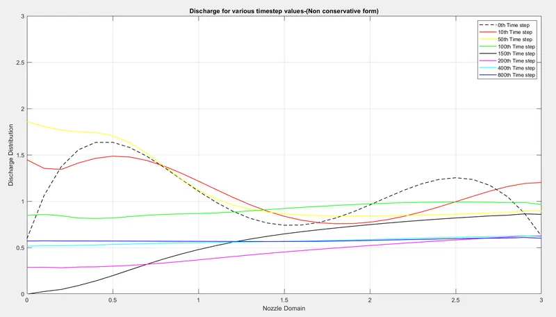
8 different curves are shown, each for a different time during the course of the time-marching procedure. The dashed curve is the variation of `rho`, V, a which pertains to the initial conditions, and hence it is labeled as 0th Time step. The
strange-looking, distorted sine like variation of this dashed curve is simply the product of the assumed initial values for `rho` and V combined with the specified parabolic variation of the nozzle area ratio A. After 50 time steps, the mass flow distribution through the nozzle has changed considerably; this is given by the curve labeled 50Llt. After 100 time steps, the mass flow distribution has changed radically; the mass flow variation is simply flopping around inside the nozzle due to the transient variation of the flow-field variables. However, after 200 time steps ,the mass flow distribution is beginning to settle down, and after 700 time steps , the mass flow distribution is a straight, horizontal line across the graph. This says that the mass flow has converged to a constant, steady-state value throughout the nozzle. This agrees with our basic knowledge of steady-state nozzle flows, namely, that `rho*v*a`= constant
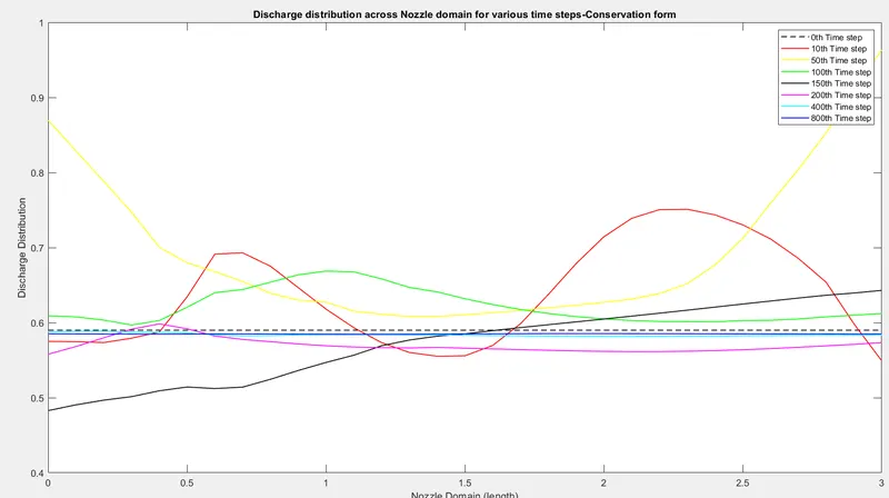
Mass flow rate distribution for various timesteps (Conservative Form)
Steady state distribution of Flow field variables (Non-Conservative form)
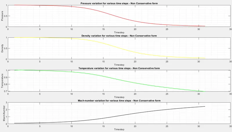
The above plot is obtained by solving the steady state values from the expression using Mccormacks Technique :
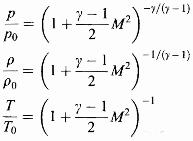
The result follows up nearly equal to the analytical results
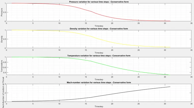
Steady state distribution of Flow field variables (Conservative form)
The above plot is obtained by solving the steady state values from the expression using Mccormacks Technique.
The result follows up nearly equal to the analytical results
Flow field variables at Throat (Non-Conservative form)
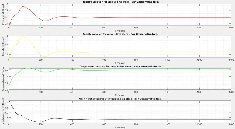
NOTE : Obtained the plot for flow field variables (primitive variables) at throat, the variables are reaching the steady state at nearly after 500 Iterations which is nearly equivalent to the analytical result, i.e after 30 to 40 ms after intiation of time step
Flow field variables at Throat (Conservative form)
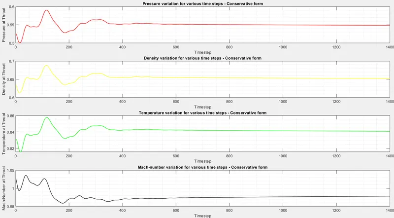
NOTE : Obtained the plot for flow field variables (primitive variables) at throat,
Able to see huge compressions and expansions of waves from time step 1 to 200 and then after 200th time step, there is one compression of pulse and then after, the waves are stretching for steady state.
The variables are reaching the steady state at nearly after 500 Iterations which is nearly equivalent to the analytical result, i.e after 30 to 40 ms after intiation of time step
Comparison of Normalised Mass flow rates of Conservative & Non- Conservative form with Analytical result :
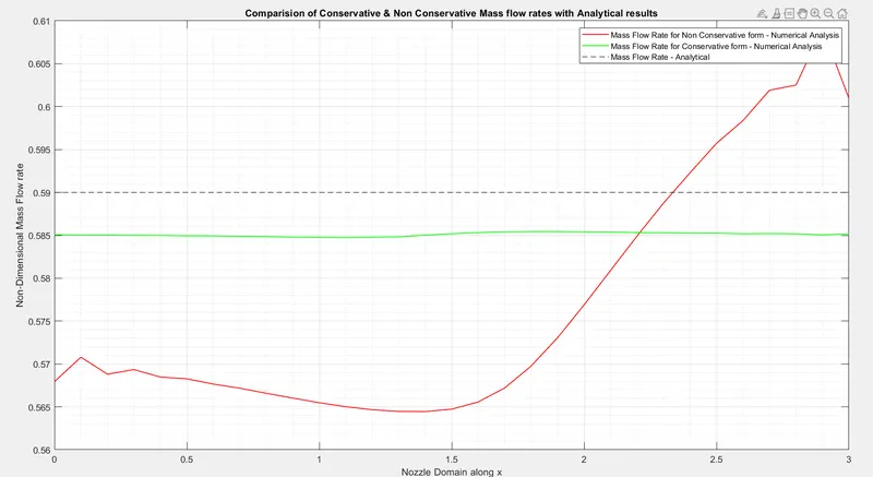
We can evidently see that Conservative form is approaching Analytical solution whereas the Non conservative form has some abrupt oscillations for inflow & outflow, indeed,because we have simulated this for a smaller scale of time step and coarser grid size.
Advantage of Conservative form :
- Conservative form is much preferred than Non-Conservative for for discharge analysis from a Quasi supersonic body
- Conservative form directly involves mass flow arte in its equation of momentum, since it is the primary output from the conservative equation
Steady State distribution of Non-dimensional density & Mach number as a function of the lengthof Nozzle :
- for x = 1.6
- Flow becomes supersonic at x >1.6
- Decrease of density due to expansion after the throat of nozzle
Residuals :
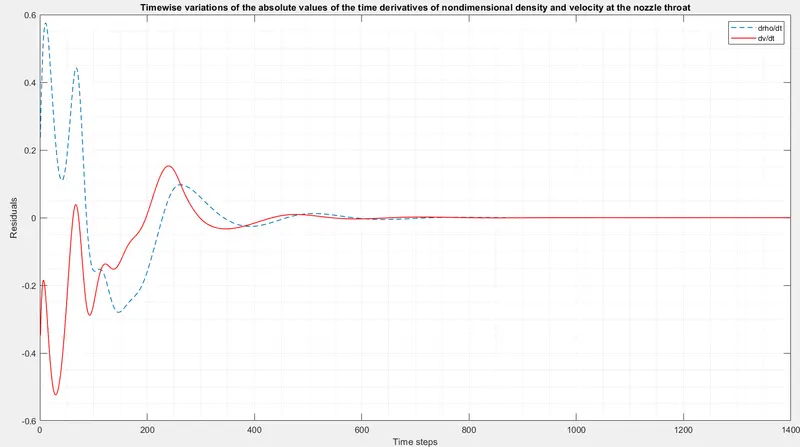
Since the numerical values of the right-hand side are not precisely zero, they are called residuals. This is why the ordinate in plot is labeled as the residual.
NOTE :
When we are comparing the relative merits of two or more different algorithms for a time-marching solution to the steady state, the magnitude of the residuals and their rate of decay are often used as figures of merit. That algorithm which gives the fastest decay of the residuals to the smallest value is usually looked upon most favorably.
For our example the decay is nearly after 600th Time step
Grid Independence Results :
| Flow field Variables (Throat) > 1000 t | Pressure | Temperature | Density | Mach Number |
| Non - Conservative form (31 Grid points) | 0.5803 | 0.8943 | 0.6489 | 0.9203 |
| Conservative form (31 Grid points) | 0.5485 | 0.8409 | 0.6523 | 0.9783 |
| Non - Conservative form (61 Grid points) | 0.5793 | 0.9110 | 0.6359 | 0.9119 |
| Conservative form (61 Grid points) | 0.5485 | 0.8409 | 0.6523 | 0.9783 |
| Analytical Results | 0.528 | 0.838 | 0.634 | 1 |
- Conservative form is approaching Analytical results for grids greater than 50, far better than Non-Conservative form
- For the non-conservative form of numerical analysis, mesh independence is achieved at 31st grid point
- Non conservative form shows a better reach for grid points less than 61