Week 5 - Rayleigh Taylor Instability

Rayleigh Taylor Instability

This is a pertained instability of two immiscible fluids, purely driven by the density stratification of two fluids. The layer between these two fluids is called "Interface"

At Base State :

This Interface is called an "Unperturbed Interface", meaning that the fluids are considered to be static in nature

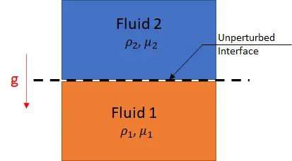
• If `rho_1 > rho_2` - Stable Configuration
• If `rho_1 < rho_2` - Unstable Configuration

Assumptions made for calculating the oscillating frequency of interface due to density stratification for Stable & Unstable cases :

• Inviscid
• Unbounded (In order to reduce BC', assume fluid extends from `(-infty) to (+infty)` in x,y & z directions

Phyical Variables

• `rho_1` - Density of Fluid 1
• `rho_2` - Density of Fluid 2
  
• `gamma` - Interfacial Tension
• g - Acceleration due to gravity

Defining a dimensionless quantity; The Atwood number is a dimensionless number in fluid dynamics used in the study of hydrodynamic instabilities in density-stratified flows

A = `[frac {rho_1-rho_2}{rho_1+rho_2}]`

Calculating the oscillating frequency of interface :

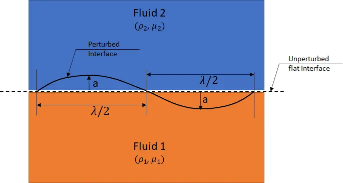
where `lamda` : Wavelength

k = `frac{2pi}{lamda}` : Wavenumber

Volume of fluid displaced/unit width (V) :

V `alpha` `[a*lamda/2*1] = [a/k]`

Net Buoyancy Force/unit width :

`F_b` `alpha` `(frac{a}{k})*(rho_2-rho_1)*g*1`

If `rho_2 >rho_1` - Destabilizing

If `rho_1 >rho_2` - Stabilizing

Surface Tension Forces :

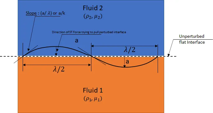
Surface tension forces tries always to pull back the perturbes interface to flat interface, the nature of Surface tension which is to minimize the surface area

Curvature of Interface : `[frac{a*k}{lamda}]` or `a*k^2`

Surface Tension `alpha` [`gamma *`curvature]

Surface Tension `alpha` [`gamma *a*k^2`]

CASE 1 : `rho_1 >rho_2` - Stabilizing Configuration

In this case both Buoyancy forces and surface tension forces are stabilizing in nature

Forces /unit width `approx` `[(gamma*a*k)] + [(frac{rho_1-rho_2}{k})*g*a]`

Volume of fluid affected due to this net force :

V `approx` `lamda^2`

Mass of fluid :

m `approx` `(rho_1 + rho_2)*lamda^2` or `frac{rho_1 - rho_2}{k^2}`

Oscillating frequency of the interface :

`omega = sqrt[frac{gamma*k^3 + (rho_1 -rho_2)*g*k}{rho_1 + rho_2}]`

CASE 2 : `rho_2 >rho_1` - Destabilizing Configuration

Forces /unit width `approx` `[(gamma*a*k)] + [(2*frac{rho_1-rho_2}{k})*g*a]`

System is unstable when :

`[(rho_2 - rho_1)/k*a*g] > 2*gamma*a*k`

or

`k^2 < frac{(rho_2-rho_1)*g}{gamma}`

Now Capillary Length (`l_c`)

`l_c = sqrtfrac{gamma}{g*(rho_2-rho_1)}`

`:.` `k <1/l_c`

Due to RT instability, any perturbation with a wavelength larger than the cutoff due to surface tension (for the immiscible case) or mass diffusion (for the miscible case) will grow.

CFD models that have been based on the mathematical analysis of Rayleigh Taylor waves

1. Kelvin-Helmholtz Instability :

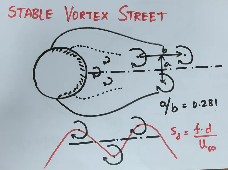
Two sheared layers are symmetrically developed forming very small vortices, this now develops to form alternative vortices on the top and bottom of the wake axis. This leaves a trail of vortices in the wake region generated in the same fashion called as Von-Karman Vortex Street. Distance between the centres of top vortices is 'a' and distance between the top and bottom vortices is 'b', Ratio of these lengths are termed as Spacing Ratio (b/a) = 0.281, termed by Von Karman.

2. Richtmyer-Meshkov instability

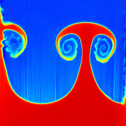
This occurs when two fluids of different density are impulsively accelerated. Normally this is by the passage of a shock wave. The development of the instability begins with small amplitude perturbations which initially grow linearly with time. This is followed by a nonlinear regime with bubbles appearing in the case of a light fluid penetrating a heavy fluid, and with spikes appearing in the case of a heavy fluid penetrating a light fluid. A chaotic regime eventually is reached and the two fluids mix. This instability can be considered the impulsive-acceleration limit of the Rayleigh Taylor instability.

3. Plateau-Rayleigh instability

This instability, often just called the Rayleigh instability, explains why and how a falling stream of fluid breaks up into smaller packets with the same volume but less surface area. It is related to the RTI and is part of a greater branch of fluid dynamics concerned with fluid thread breakup. This fluid instability is exploited in the design of a particular type of ink jet technology whereby a jet of liquid is perturbed into a steady stream of droplets. The driving force of the Plateau–Rayleigh instability is that liquids, by virtue of their surface tension, tend to minimize their surface area.

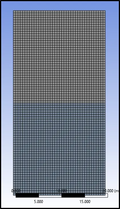
Geometry creation and conformal mesh creation :

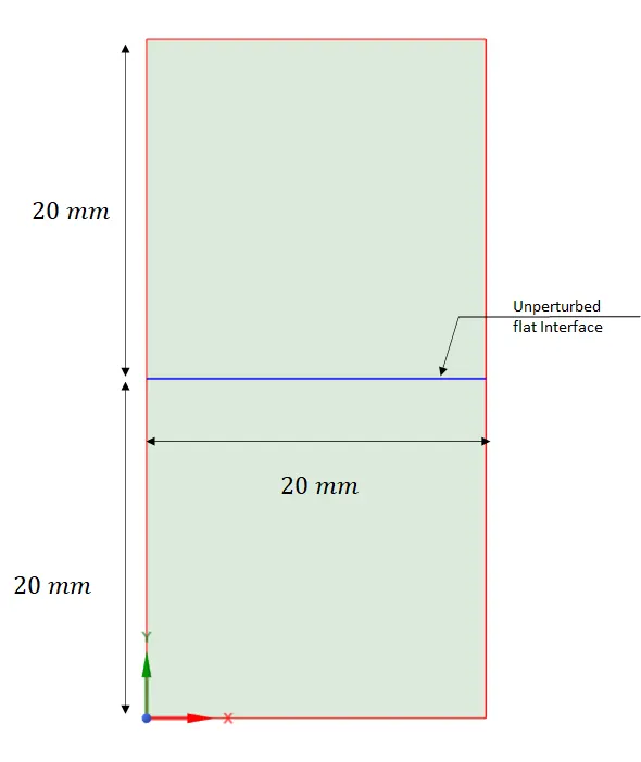
Create a geometry of 20mm x 20mm for both fluids one above the other.

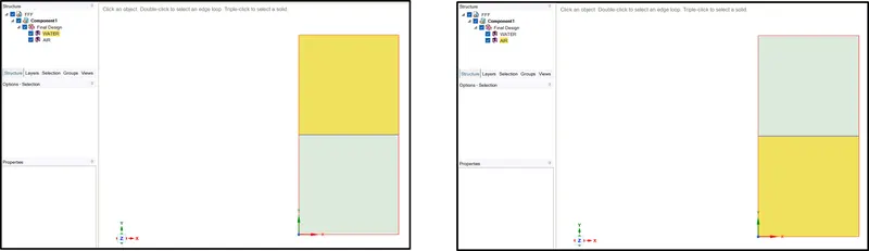
Go to Structures and create a seperate folder for storing these components as Air and water

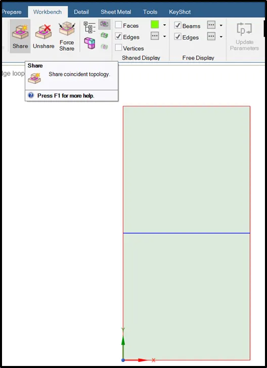
Conformal Meshing :

Then Go to Workbench > Share Topology for making the interface transfer information from cell to other

Mesh Generation :

• Structured Grid

• Element Size

a) Case 1 : 0.5 mm

b) Case 2 : 0.3 mm

Physics Setup :

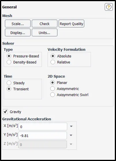
General > Pressure based > Transient > Gravity > y = -9.81m/s2

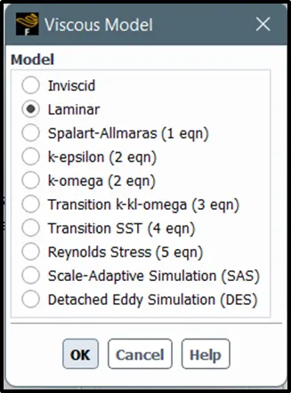
Viscous Model > Laminar

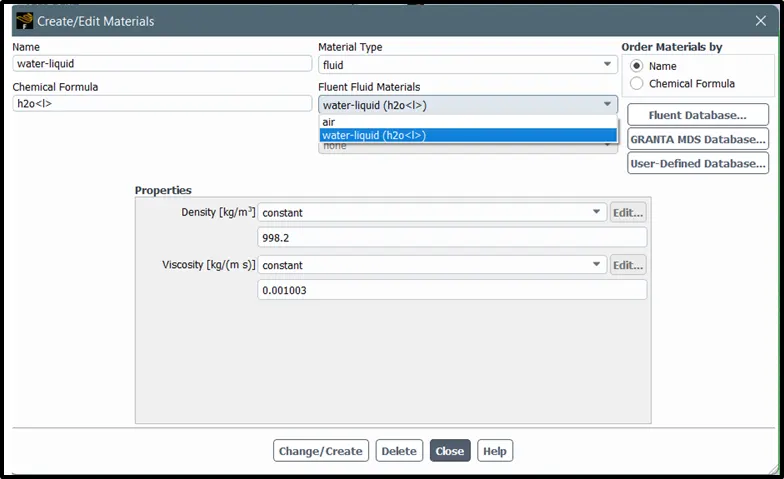
Materials > Fluent Database (To add water) > Scroll down to water (Liquid) > Copy > Close

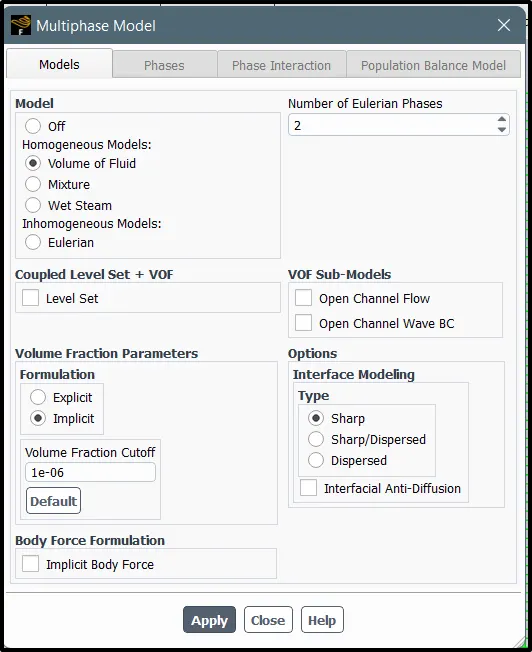
Go to Multiphase > Models > Volume of Fluid > Volume fraction parameters > Implicit

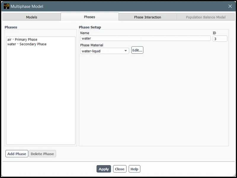
Go to Multiphase > Phases > Models > Change phase setup name for air as "air" > Change phase setup name for water-liquid as "water"

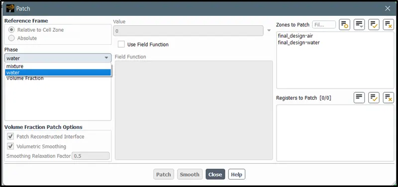
Now Initialize the solution > Entering Patching

Select Phases >Water > Go to Zones to patch > Select water design > Change value to 1 > Patch > Then select air design > Change value to 0 > Patch > Close

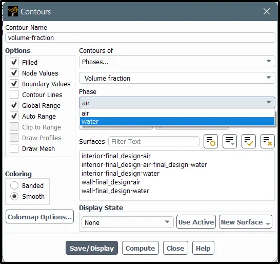
Go to Results > Contours > New

Results and observations :

Case 1 : Grid size 0.3mm of air & water

Simulation Video Link :https://drive.google.com/file/d/1FHSOdRjU6X61Bz-tVlBsMCTZ6ox6kgZZ/view?usp=sharing

Case 2 : Grid size 0.5mm of air & water

Simulation Video Link :https://drive.google.com/file/d/1FPxh5ZTWzGulV2l0i1jbII9tv6k5YvhI/view?usp=sharing

Case 3 : Grid size 0.5mm of air & UDF

Simulation Video Link :https://drive.google.com/file/d/1P43nmuw4i5i5cY1ScHTkOj79ijisbrOx/view?usp=sharing

Atwood Number Calculation :

A = `[frac {rho_1-rho_2}{rho_1+rho_2}]`

For CASE 1:

`rho_1` = 998.2`(kg)/m^3`

`rho_2` = 1.225`(kg)/m^3`

A = `[frac{998.2-1.225}{998.2+1.225}]`

A = 0.99754 `approx`1

For CASE 2:

`rho_1` = 998.2`(kg)/m^3`

`rho_2` = 400`(kg)/m^3`

A = `[frac{998.2-400}{998.2+400}]`

A = 0.42783 `approx`0.43

Conclusions :

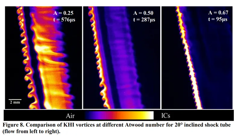
• Growth Rate of Instabilities increases as the Atwood Number Increases
• This corresponds to larger wavelengths for lower Atwood numbers

Reference of dependancy of this data:

Effects of Atwood number on Kelvin-Helmholtz Instabilities Formed from Oblique Shock Interaction with a Heavy Gas Column - Jason H. Yoo1
The University of New Mexico, Albuquerque, New Mexico, 87131