Week 4.1 - Genetic Algorithm
AIM: To optimize a stalagmite Function using Genetic Algorithm
Theory of Genetic Algorithm:
A genetic algorithm (GA) is a method for solving both constrained and unconstrained optimization problems based on a natural selection process that mimics biological evolution.
Computational way of understanding the Genetic Algorithm involves Chromosomes as the solutions to the set of equations with unknown variables. Set of Chromosomes forms a population. In order to keep the species alive, chromosomes have to reproduce the next chromosomes. Hence two chromosomes for mating should be fittest to survive the nature among other chromosomes & mate to produce new chromosome. A new chromosome can also undergo mutation according to required surviving characteristics.
Genetic Algorithm:
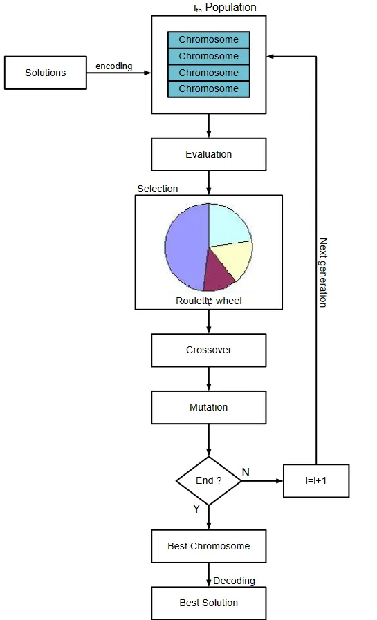
Pseudo Code for Genetic Algorithm :
STEP I : Initialize Random Population(P);
STEP II : Evaluate fitness(f) of Population(P);
STEP III : Exterior Iteration Loop
for t = 1 to T ; where T is the number of generations the algorithm has to iterated before termination.
STEP IV : Perform Tournament selection of Tournament Size (k)
Assuming k = 2
CrossOver Operator Iteration Loop :
for i = 1:Np/2 where Np is the random population and this loop selects even random numbers of 2;
if r`<=`Pc (Probability of Crossover);
Perform Crossover over the selected numbers;
else
Copy selected parents & fitness to offspring population
end
STEP V : Perform Polynomial Mutation of ith solution :
for i = 1:Np
if r`<=`Pm (Probability of Mutation);
Perform Polynomial Mutation over the selected numbers;
else
No changes in ith solution of offspring
end
STEP VI : Evaluate Fitness
Syntax for ga in MatLab
X = ga(fun, nvars, A, B, Aeq, Beq, lb, ub, nonlcon, options);
fun - Function to be optimised
nvars - Number of Variables of the function
A - Linear Inequalities
B - Linear Inequalities
Aeq - Linear Equalities
Beq - Linear Equalities
lb - lower Bounds
ub - upper bounds
nonlcon - non linear constraints
options - options to optimize ga function
NOTE : "ga" is an inbuilt matlab function which is utilized for optimisation of trial functions to find global minimas and maximas.
This function chooses random numbers everytime hence every time this function is executed it provides us diffrent results. In order to eliminate this, the lb (lower bound) values & ub (upper bound) values are utilized to compress output optimized function to suitable range.
ga function has another inbuilt attribute. This iterates the optimization for population size of 50 as default, i.e it iterates the results for 50 generations & then terminates the function execution.
We can manipulate this behaviour of 'ga' by using options as of a syntax in ga to increase the population size to any number. This inturn optimizes the solution to a near accuracy. CASE 3 in the coding given below is a fine example of Increasing population size and we can witness the utmost optimised result.
MatLab code for Optimisation of Stalagmite Function :
%% Stalgmite Function against x & y:
clear
close
clc

x = linspace(0,0.6,150);
y = linspace(0,0.6,150);

[X , Y] = meshgrid(x,y);

for i = 1:length(X)
    for j = 1:length(Y)

        input_vector(1) = X(i,j);
        input_vector(2) = Y(i,j);
        f(i,j) = stalagmite(input_vector);
    end
end

surf(X,Y,f);

shading interp

xlabel('X Axis');
ylabel('Y Axis');
zlabel('Z Axis');

______________________________________________________________________________________

%% Optimisation of Stalgmite function using Genetic Algorithm (ga) for Statistical Behaviour

% CASE 1: Unbounded Input values for ga

% Defining x & y:

x = linspace(0,0.6,150);
y = linspace(0,0.6,150);

[X,Y] = meshgrid(x,y);

% No of generations the ga must be iterated (T);
T = 50; % Default population size captured by ga.


% Studying ga for Statistical Analysis
% Study 1 (For Unbounded Values)

% Evaluation of Code Run time
tic
for i = 1:T
    [inputs,fopt(i)] = ga(@stalagmite,2);
    % ga is an inbuilt function
    % ga(fun,nvars) is the syntax for this function


    xopt(i) = inputs(1);
    yopt(i) = inputs(2);
end
study1_time = toc;

% Plotting the all the optimum values in the same figure window

figure(1)
subplot(2,1,1)
% Tool that helps us plot multiple plots inside a same figure window
% Syntax - subplot(m,n,p) where
% "m" is the no of rows in the figure window,
% "n" is the no of colums in the figure window
% "p" is the row number where this plots exists
hold on
surf(x,y,-f);
shading interp
plot3(xopt,yopt,-fopt,'marker','o','markersize',5,'markerfacecolor','r');
title('Unbounded Inputs');

subplot(2,1,2)
plot(-fopt);
xlabel('Iterations');
ylabel('Function Minimum')

______________________________________________________________________________________


%% Optimisation of Stalgmite function using Genetic Algorithm (ga) for Statistical Behaviour

% CASE 2 : Bounded Input values for ga

% Study 2 (Bounded Values)


% Iteration Loop
tic
for i = 1:T
    [inputs,fopt(i)] = ga(@stalagmite,2,[],[],[],[],[0;0],[1;1]);
    % ga is an inbuilt function
    % ga(fun,nvars) is the syntax for this function


    xopt(i) = inputs(1);
    yopt(i) = inputs(2);
end
study2_time = toc;

% Plotting the all the optimum values in the same figure window

figure(2)
subplot(2,1,1)
% Tool that helps us plot multiple plots inside a same figure window
% Syntax - subplot(m,n,p) where
% "m" is the no of rows in the figure window,
% "n" is the no of colums in the figure window
% "p" is the row number where this plots exists
hold on
surf(x,y,-f);
shading interp
plot3(xopt,yopt,-fopt,'marker','o','markersize',5,'markerfacecolor','r');
title('Bounded Inputs');

subplot(2,1,2)
plot(-fopt);
xlabel('Iterations');
ylabel('Function Minimum')


______________________________________________________________________________________


%% %% Optimisation of Stalgmite function using Genetic Algorithm (ga) for Statistical Behaviour

% CASE 3 : Bounded Input values for ga & Increasing no of generations from 50 to 250

% Study 3 (Increasing T)

options = optimoptions('ga');
% Optimzations tool syntax of ga for increasing accuracy rate
% optimizations can be done to "ga","integer ga" & "gamultiobj"
% Syntax for Options :
% Options = optimoptions(solvername,Name,Size);
options = optimoptions(options,'PopulationSize',200);

% Iteration Loop
tic
for i = 1:T
    [inputs,fopt(i)] = ga(@stalagmite,2,[],[],[],[],[0;0],[1;1],[],[],options);
    % ga is an inbuilt function
    % ga(fun,nvars) is the syntax for this function


    xopt(i) = inputs(1);
    yopt(i) = inputs(2);
end
study3_time = toc;

% Plotting the all the optimum values in the same figure window

figure(3)
subplot(2,1,1)
% Tool that helps us plot multiple plots inside a same figure window
% Syntax - subplot(m,n,p) where
% "m" is the no of rows in the figure window,
% "n" is the no of colums in the figure window
% "p" is the row number where this plots exists
hold on
surf(x,y,-f);
shading interp
plot3(xopt,yopt,-fopt,'marker','o','markersize',5,'markerfacecolor','r');
title('Increased Population Size');

subplot(2,1,2)
plot(-fopt);
xlabel('Iterations');
ylabel('Function Minimum')
Explaination of Code:
1. Defining Stalgmite Function:
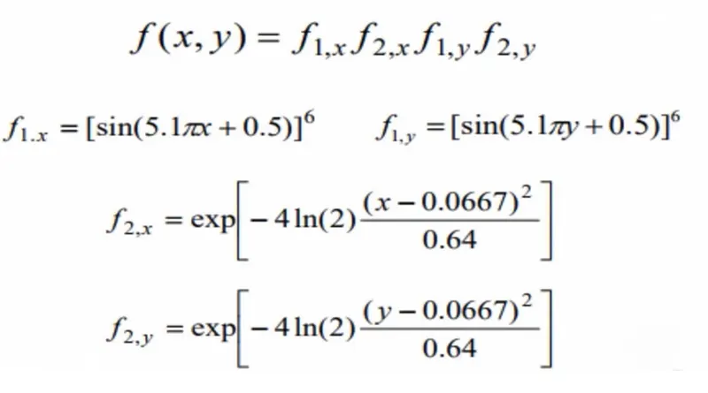
2. Defining variables x & y and defining no of generations (T), ga has to iterate .
3. CASE I Study:
Iterative loop to be formed using for loop with counter from 1 to T
4. ga function is called for optimising stalagmite function of 2 variables x & y;
5. optimum values for x & y are defined & study time is calculated using tic & toc
Plotting
6. Inorder to have multiple plots inside same figure window we can use 'subplot'
Syntax for subplot
subplot(m,n,p) where
m is no of rows inside fig window,
n is no of colums inside fig window &
p is the row number for respective figure
7. Inorder to visualize the plot we can use 'surfc' command for x, y & f as a 3d quantity visualization
8. We plot 3d quantities using 'plot3' command for plotting the optimum values using markers
9. A second plot inside the same figure window is made for f optimum using 'plot' command
CASE II Study:
Iterative loop to be formed using for loop with counter from 1 to T
1. ga function is called for optimising stalagmite function of 2 variables x & y with upper & lower bound limits
2. optimum values for x & y are defined & study time is calculated using tic & toc
Plotting
3. Inorder to have multiple plots inside same figure window we can use 'subplot'
Syntax for subplot
subplot(m,n,p) where
m is no of rows inside fig window,
n is no of colums inside fig window &
p is the row number for respective figure
4. Inorder to visualize the plot we can use 'surfc' command for x, y & f as a 3d quantity visualization
5. We plot 3d quantities using 'plot3' command for plotting the optimum values using markers
6. A second plot inside the same figure window is made for f optimum using 'plot' command
CASE III Study:
Iterative loop to be formed using for loop with counter from 1 to T
1. ga function is called for optimising stalagmite function of 2 variables x & y with upper & lower bound limits & Increased Iterations using Options
2. optimum values for x & y are defined & study time is calculated using tic & toc
Plotting
3. Inorder to have multiple plots inside same figure window we can use 'subplot'
Syntax for subplot
subplot(m,n,p) where
m is no of rows inside fig window,
n is no of colums inside fig window &
p is the row number for respective figure
4. Inorder to visualize the plot we can use 'surfc' command for x, y & f as a 3d quantity visualization
5. We plot 3d quantities using 'plot3' command for plotting the optimum values using markers
6. A second plot inside the same figure window is made for f optimum using 'plot' command
RESULTS
CASE I : Unbounded Plots with 50 Iterations
Trial I
Trial II
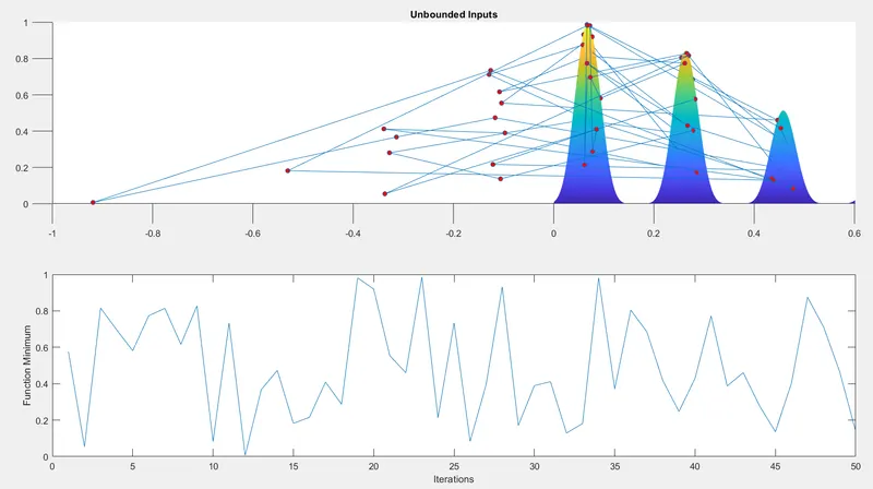
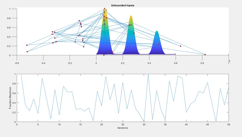
We clearly witness that ga is selecting the values differently & varies beyond 0 & 0.6, eventhough the limits are given in defining the variables x & y. The study time is still insignificant
Hence in order to limit the ga optimised output we have to include limits in its syntax of lb (lower bound) & ub (upper bound).
CASE II : Bounded Plots with 50 Iterations
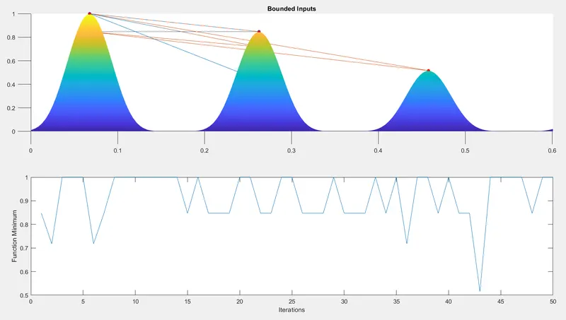
We clearly witness that ga is not varying beyond 0 & 0.6 since we have mentioned lb & ub in ga. The study time is still insignificant & the results are not yet accurately optimised as we still see multiple local maximas
Hence in order to have a accuarate optimization we have to increase the iteration number by utilizing 'options' .
CASE III : Bounded Plots with Increased Iterations
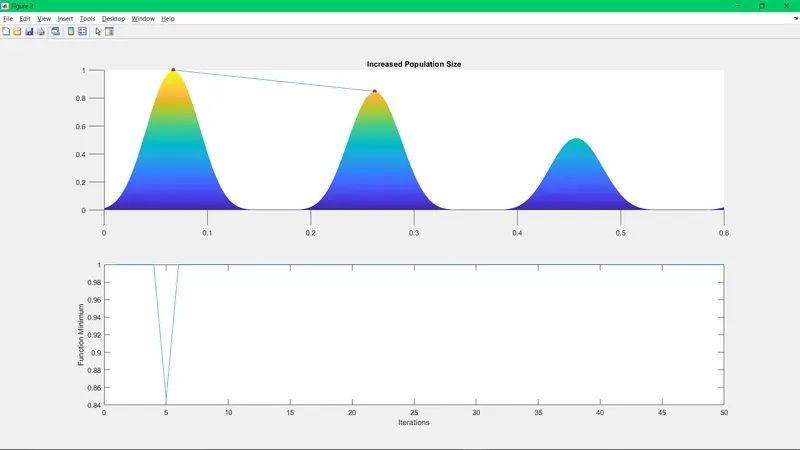
We clearly witness only one Global Maxima in this case since we have increased the iterations. Clearly we also witness a significant increase in Study time for this case.
Errors while coding :
1. Incorret Syntax Usage of ga
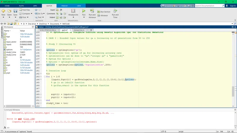
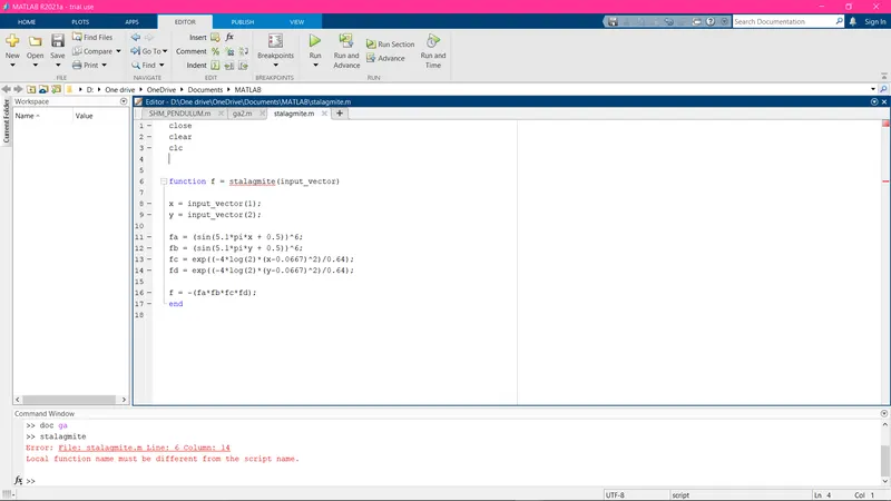
2. Usage of Clear, close & clc during defining function