Week 5.1 - Mid term project - Solving the steady and unsteady 2D heat conduction problem
Solving the steady and unsteady 2D heat conduction problem :
Governing Differential equation for Heat Conduction
`rho*C_p*(frac{delT}{delt}) + beta*T* (frac{delP}{delt}) = frac{del}{delx}*k_x(frac{delT]{delx}) + frac{del}{dely}*k_y(frac{delT]{dely}) + frac{del}{delz}*k_z(frac{delT]{delz}) + Q''' => (star)`
where
`rho` is the density of the medium in conduction
`c_p` is the specific heat capacity of the medium in conduction
`k_x , k_y & k_z ` are the Thermal Conductivities of the medium in x, y & z direction respectively
`Q'''` is the rate of heat generated by the medium per unit volume
`beta` is the volumetric co-efficient of the medium
`frac{delp}{delt}` is the compressibilty of the medium
Assumptions for Heat Conduction in solids :
1. For Conduction in solids as Volumteric Coefficient `beta < < <1` and compressibility of solids is nearly 0
2. Considering an Isotropic material of solid which tends to produce equal thermal conductivity in all directions
`:. k_x = k_y = k_z = k`
After these assumptions, the equation boils down to :
`rho*C_p*(frac{delT}{delt}) = frac{del}{delx}*k(frac{delT]{delx}) + frac{del}{dely}*k(frac{delT]{dely}) + frac{del}{delz}*k(frac{delT]{delz}) + Q'''`
but we can rewrite pde's of spatial temperature derivatives in Laplacian Form as
`frac{del}{delx}*k(frac{delT]{delx}) + frac{del}{dely}*k(frac{delT]{dely}) + frac{del}{delz}*k(frac{delT]{delz}) = k*(nabla^2*T)`
`:. rho*C_p*(frac{delT}{delt}) = k*(nabla^2*T) + Q'''`
3. Assuming no heat generation from the solid body
`rho*C_p*(frac{delT}{delt}) = k*(nabla^2*T)->`Unsteady State no heat generation 3D Heat Conduction equation
Now : For solids `C_p = C_v = C`
where `[frac{k}{rho*C}] = alpha` which is the Thermal Diffusivity of the material
`(frac{delT}{delt}) = alpha*k*(nabla^2*T)`
Thermal Diffusivity can also be realised by Ability to conduct heat /Ability to store heat
4. Assuming that temperature is constant with time marching forward, the equation boils down to
`frac{delT}{delt} = 0;`
`:. k*(nabla^2*T) = 0 ->` Steady state no heat generation 3D Heat Conduction equation
Discretization & solving steady state 2-D heat conduction equation for an isotropic solid body :
2-D Steady State Heat Conduction Equation :
`[frac{del}{delx}*k*frac{delt]{delx}] + [frac{del}{dely}*k*frac{delt]{dely}] = 0`
`(frac{del^2T}{delx^2} + frac{del^2T}{dely^2}) = 0 -> (1)`
Evaluating temperatute Tp at the centre of the plate using dicretized Heat conduction equation by Central Difference Scheme :
Let us consider a flat plate with dimension (X*Y) as an area with each side subdivided into 2 sections by three nodes one each side. Distance between nodes in X direction be `DeltaX` & distance between nodes in X direction be `DeltaY`.
`et `T_P` be the temperature at the centre of the plate which is to be determined using Heat conduction equation. The temperature at the top, bottom, left & right are given below as follows`
1. `T_T` = 600K
2. `T_B` = 900K
3. `T_L` = 400K
4. `T_R` = 800K
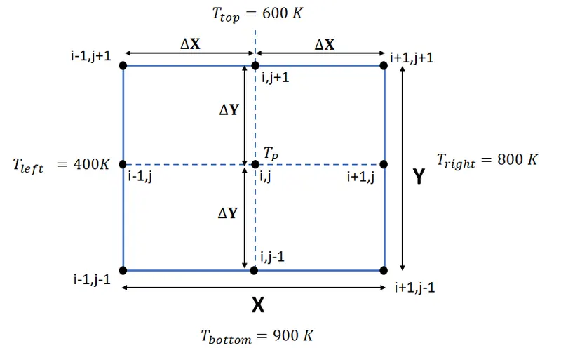
Space Marching Problem :
Applying Central Difference Scheme to find the value of `T_P`
`[frac{T_L -2T_P+T_R}{DeltaX^2}] +[frac{T_T -2T_P +T_B}{DeltaY^2}]=0`
`frac{2T_P}{DeltaX^2} + frac{2T_P}{DeltaY^2} = [frac{T_L +T_R}{DeltaX^2}]+[frac{T_T + T_B}{DeltaY^2}]`
`T_P*(frac{2*(DeltaX^2+DeltaY^2)}{DeltaX^2*DeltaY^2}) = [frac{T_L +T_R}{DeltaX^2}]+[frac{T_T + T_B}{DeltaY^2}]`
Now we can assign a value k = `(frac{2*(DeltaX^2+DeltaY^2)}{DeltaX^2*DeltaY^2})`
`:. T_P*(k) = [frac{T_L +T_R}{DeltaX^2}]+[frac{T_T + T_B}{DeltaY^2}]`
Expressing Temperatures in using co-ordinates of (i,j) :
`T_(i,j) = 1/k*[frac{T_((i-1,j)) +T_((i+1,j))}{DeltaX^2}]+[frac{T_((i, j-1)) + T_((i,j+1))}{DeltaY^2}]`
Coding procedure and strategy followed :
1. Defining the domain, number of grid points & size of the grid
2. Calculating Grid Size along X & Y
3. Creating 2-D array
4. Initializing Temperature "t" & applying BC's
5. Applying BC's
6. Assigning corner temperatures
7. Initialising while loop condition data for iterations
8. Initialising temperatures for all three solvers
9. Initialising Loop counters for all three solvers
10. Assigning an Input 'Schemes' giving the user a choice to choose the solver type
11. Calculating t(i,j) using 'for loop' for i & j of nodes running from 2 to n-1
12. Calculating Error of `T_(o l d)` from T
13. Updating `T_(o l d)`
14. Contour plotting
MatLab Code to calculate T :
%% Calculating T_p for 2-D Steady State Heat Conduction Equation
 clear
 close all
 clc

 %% Defining the domain, number of grid points & size of the grid

 % Number of grid points along X :
 nx = 10;

 % Number of grid points along y :
 ny = 10;

 % Defining the domain length of X :
  x = linspace(0,1,nx);

 % Defining the domain length of y :
  y = linspace(0,1,ny);

 % Flipping the y array :

 % Calculating Grid Size along X :
 dx = 1/(nx-1);

 % Calculating Grid Size along y :
 dy = 1/(ny-1);

 % Defining K :
 K = (2*(dx^2 + dy^2)/(dx^2*dy^2));

%% Initializing Temperature "t" & applying BC's:

t = 300*ones(nx,ny);

% Applying BC's :

 t(1,:)=900;
 t_t = 900;
 t(end,:)=600;
 t_b = 600;
 t(:,1)=400;
 t_l = 400;
 t(:,end)= 800;
 t_r = 800;

 % Assigning corner temperatures
 t(1,1) = (t_t + t_l)/2;
 t(1,end) = (t_t + t_r)/2;
 t(end,end) = (t_b +t_r)/2;
 t(end,1) = (t_l +t_b)/2;


 %% Calculation of T(i,j) using JACOBIAN,GS & SOR

 tol = 1e-4; % Defining threshold error

 error = 1; % Initializing the value of error so that while loop starts

% Creating copy of t
 told = t;
 t_ini = t;

%  tic        % Computing Run time
 iter = 1;  % Intializing Loop counter

            while(error > tol)
                for i=2:nx-1
                for j=2:ny-1
                   t(i,j) = (1/(K))*((told((i+1),j) + told((i-1),j))/(dx^2)) + (1/(K))*((told(i,(j+1)) + told(i,(j-1)))/(dy^2));
                end
                end

                 % Calculating error
                 error = max(max(abs(told -t)));

                 % Updating T
                 told = t;
                 iter = iter +1;
                 [XX,YY] = meshgrid(x,y);

                     set(gca,'ydir','reverse');
                     contourf(XX,YY,t); % Using Contour command to plot
                     colormap(jet);
                     [C,h] = contourf(XX,YY,t); % Using 'clabel' labels the current contour plot with rotated text inserted into each contour line
                     clabel(C,h)
                     colorbar;
                     xlabel('Domain of along X')
                     ylabel('Domain of along Y')
                     run_time = toc ;
                     title_text2 = sprintf('No of iterations to converge using Jacobi Iteration solver = %d',iter);
                     title({'STEADY STATE NON HEAT GENERATION 2-D HEAT CONDUCTION TEMP PROFILE';title_text2});
                     pause(0.001);


            end
Results : Jacobian Iterative Method
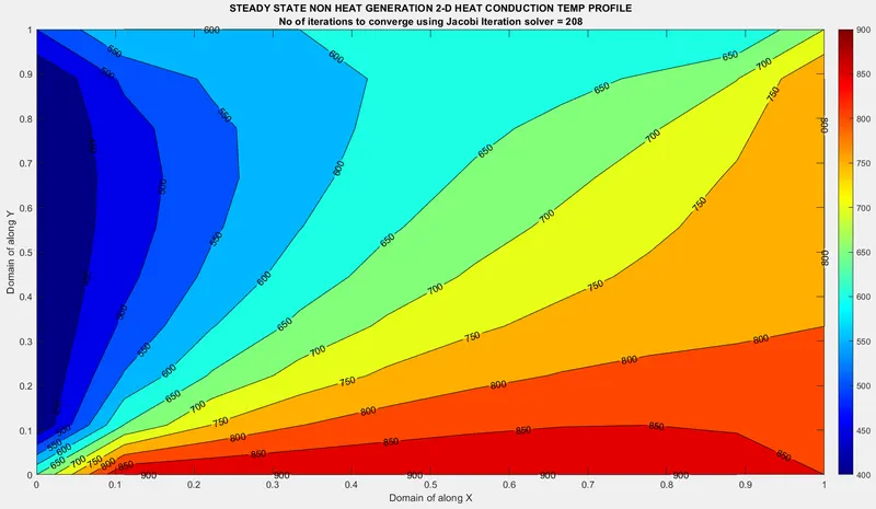
Solving Transient/Unsteady state 2-D heat conduction equation for an isotropic solid body :
`rho*C_p*(frac{delT}{delt}) = k*(nabla^2*T)->`Unsteady State no heat generation 3D Heat Conduction equation
Now : For solids `C_p = C_v = C`
where `[frac{k}{rho*C}] = alpha` which is the Thermal Diffusivity of the material
`(frac{delT}{delt}) = alpha*k*(nabla^2*T)`
Thermal Diffusivity can also be realised by Ability to conduct heat /Ability to store heat
Time Marching Problem :
Explicit Scheme = `T_P^(n-1) = T_P^(n)*(1-2K1-2K2) + K1*(T_L^(n) +T_R^(n)) + K2*(T_B^(n) +T_T^(n))`
1) Jacobian Iterative Method = `T_P^(n+1) = frac{T_P + K1(T_L^n + T_R ^n) + K2(T_T^n + T_B^n)}{1+2K1+2K2}`
2) Gauss Seidal Method = `T_P^(n+1) = frac{T_P + K1(T_L^(n+1) + T_R ^n) + K2(T_T^(n+1) + T_B^n)}{1+2K1+2K2}`
3) Successive Over relaxation = `T_P^(n+1) = omega* frac{T_P + K1(T_L^(n+1) + T_R ^n) + K2(T_T^(n+1) + T_B^n)}{1+2K1+2K2}`
Coding procedure and strategy followed :
1. Defining the domain, number of grid points & size of the grid
2. Calculating Grid Size along X & Y
3. Creating 2-D array
4. Initializing Temperature "t" & applying BC's
5. Applying BC's
6. Assigning corner temperatures
7. Initialising while loop condition data for iterations
8. Initialising temperatures for all three solvers
9. Initialising Loop counters for all three solvers
10. Assigning CFL Condition for stability of solution
11. Assigning an Input 'Schemes' giving the user a choice to choose the solver type
12. Calculating t(i,j) using 'for loop' for i & j of nodes running from 2 to n-1
13. A time loop to be included with counter running from 1 to nt
14. Calculating Error of `T_(o l d)` from T
15. Updating `T_(o l d)`
16. Contour plotting
Matlab code to evaluate T using all solver techniques :
% Calculating T_p for 1-D Steady State Heat Conduction Equation
 clear
 close all
 clc

 %% Defining the domain, number of grid points & size of the grid

 % Number of grid points along X :
 nx = 10;

 % Number of grid points along y :
 ny = 10;

 % Defining the domain length of X :
  x = linspace(0,1,nx);

 % Defining the domain length of y :
  y = linspace(0,1,ny);

 % Flipping the y array :

 % Calculating Grid Size along X :
 dx = 1/(nx-1);

 % Calculating Grid Size along y :
 dy = 1/(ny-1);

 % Creating 2-D array :
 [XX,YY] = meshgrid(x,y);

 % Defining K :
 K = (2*(dx^2 + dy^2)/(dx^2*dy^2));

 % Relaxation Factor
  omega = 0;

 % Initializing Temperature "t" & applying BC's:

 t = 300*ones(nx,ny);

 % Applying BC's :
 t(1,:)=900;
 t_t = 900;
 t(end,:)=600;
 t_b = 600;
 t(:,1)=400;
 t_l = 400;
 t(:,end)= 800;
 t_r = 800;

 % Assigning corner temperatures
 t(1,1) = (t_t + t_l)/2;
 t(1,end) = (t_t + t_r)/2;
 t(end,end) = (t_b +t_r)/2;
 t(end,1) = (t_l +t_b)/2;

 % Initialising data for iterations
 error = 1;        % Initialising error
 tol = 1e-4;       % Threshold limit of error

 % Initialising temperatures for all three solvers
 told = t;
 told2 = t;
 told3 = t;
 tp = t;
 t_initial = t;

 % Initialising Loop counters for all three solvers
 j_iter = 1;
 gs_iter = 1;
 sor_iter = 1;

 % CFL Condition for stability of solution
 a = 1; %  Thermal Diffusivity
 int_time = 10; % Integration Time
 dt = 2; % Time step
 nt = int_time/dt; % Total no of times calculations are performed
 c = (a*(dt))/(dx^2);
 c2 = (a*(dt))/(dy^2);

  % Input Schemes
 scheme = input('Enter Scheme 1.Explicit 2.Implicit Jacobi 3.Implicit GS 4.Implicit SOR');

 %% For Transient Explicit Scheme

 if (scheme==1)
     int_time = 10;
     dt = 0.1;
     nt = int_time/dt;
     a = 0.01;
     c = (a*dt)/(dx^2);
     c2 = (a*(dt))/(dy^2);

     j_iter = 1;
       for u = 1:nt
           for i = 2:nx-1
               for j = 2:ny-1
                   term1 = (told(i-1,j))-(2*told(i,j))+(told(i+1,j));
                   term2 = (told(i,j-1))-(2*told(i,j))+(told(i,j+1));
                   t(i,j)= told(i,j)+(c*term1)+(c2*term2);
               end
           end

           % Calculating Error
           error = max(max(abs(told - t)));

           % Updating told
           told = t ;
           j_iter = j_iter+1;

           % Contour Plotting & Evaluating no of iterations
                     set(gca,'ydir','reverse');
                     contourf(XX,YY,t); % Using Contour command to plot
                     colormap(jet);
                     [C,h] = contourf(XX,YY,t); % Using 'clabel' labels the current contour plot with rotated text inserted into each contour line
                     clabel(C,h)
                     colorbar;
                     xlabel('Domain of along X')
                     ylabel('Domain of along Y')
                     title_text1 = sprintf('No of iterations to converge using Explicit Scheme = %d',j_iter);
                     title({'TRANSIENT STATE 2-D HEAT CONDUCTION TEMP PROFILE';title_text1});
                     pause(0.001);
       end
 end


 % For Transient Implicit (Jacobian Iteration Scheme)

 if (scheme==2)

     j_iter = 1;
     for v = 1:nt % Time Loop
         while error > tol
             for i = 2:nx-1
                 for j = 2:ny-1
                     term1 = (1+(4*c))^-1;
                     term2 = c2*term1;
                     F = (told(i-1,j) + told(i+1,j));
                     G = (told(i,j-1) + told(i,j+1));
                     t(i,j) = (tp(i,j)*term1)+(F*term2)+(G*term2);
                 end
             end

            % Calculating Error
             error = max(max(abs(t-told)));

             % Upldating value of Error
             told = t;

             j_iter = j_iter +1;

                % Contour Plotting & Evaluating no of iterations
                     set(gca,'ydir','reverse');
                     contourf(XX,YY,t); % Using Contour command to plot
                     colormap(jet);
                     [C,h] = contourf(XX,YY,t); % Using 'clabel' labels the current contour plot with rotated text inserted into each contour line
                     clabel(C,h)
                     colorbar;
                     xlabel('Domain of along X')
                     ylabel('Domain of along Y')
                     title_text1 = sprintf('No of iterations to converge using Implicit Jacobian Scheme = %d',j_iter);
                     title({'TRANSIENT STATE 2-D HEAT CONDUCTION TEMP PROFILE';title_text1});
                     pause(0.001);
         end
         tp = told;

     end
 end


  %% For Transient Implicit (Gauss-Seidal Iteration Scheme)

 if (scheme==3)

     gs_iter = 1;
     for w = 1:nt % Time Loop
         while error > tol
             for i = 2:nx-1
                 for j = 2:ny-1
                     term1 = (1+(4*c))^-1;
                     term2 = c2*term1;
                     F = (t(i-1,j) + told2(i+1,j));
                     G = (t(i,j-1) + told2(i,j+1));
                     t(i,j) = (tp(i,j)*term1)+(F*term2)+(G*term2);
                 end
             end

            % Calculating Error
             error = max(max(abs(t-told2)));

             % Upldating value of Error
             told2 = t;

             gs_iter = gs_iter +1;

                % Contour Plotting & Evaluating no of iterations
                     set(gca,'ydir','reverse');
                     contourf(XX,YY,t); % Using Contour command to plot
                     colormap(jet);
                     [C,h] = contourf(XX,YY,t); % Using 'clabel' labels the current contour plot with rotated text inserted into each contour line
                     clabel(C,h)
                     colorbar;
                     xlabel('Domain of along X')
                     ylabel('Domain of along Y')
                     title_text1 = sprintf('No of iterations to converge using Implicit Gauss-Seidal Scheme = %d',gs_iter);
                     title({'TRANSIENT STATE 2-D HEAT CONDUCTION TEMP PROFILE';title_text1});
                     pause(0.001);
         end
         tp = told;

     end
 end


 %% For Transient Implicit (Successive Over Relaxation Iteration Scheme)

 if (scheme==4)
     omega = input('Enter relaxation factor');

     sor_iter = 1;
          for o = 1:nt % Time Loop
         while error > tol
             for i = 2:nx-1
                 for j = 2:ny-1
                     term1 = (1+(4*c))^-1;
                     term2 = c*term1;
                     F = (t(i-1,j) + told3(i+1,j));
                     G = (t(i,j-1) + told3(i,j+1));
                     t(i,j) = (tp(i,j)*term1)+ (F*term2)+ (G*term2);
                     t(i,j) = (1-omega)*told3(i,j)+omega*t(i,j);
                 end
             end

            % Calculating Error
             error = max(max(abs(t-told3)));

             % Upldating value of Error
             told3 = t;

             sor_iter = sor_iter +1;


                % Contour Plotting & Evaluating no of iterations
                     set(gca,'ydir','reverse');
                     contourf(XX,YY,t); % Using Contour command to plot
                     colormap(jet);
                     [C,h] = contourf(XX,YY,t); % Using 'clabel' labels the current contour plot with rotated text inserted into each contour line
                     clabel(C,h)
                     colorbar;
                     xlabel('Domain of along X')
                     ylabel('Domain of along Y')
                     title_text1 = sprintf('No of iterations to converge using Implicit SOR Scheme = %d',sor_iter);
                     title({'TRANSIENT STATE 2-D HEAT CONDUCTION TEMP PROFILE';title_text1});
                     pause(0.001);
         end
         tp = told;

          end
 end
Results :
(1) Explicit Scheme
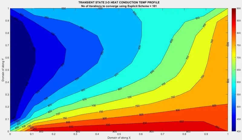
(2) Implicit Scheme (Jacobian)
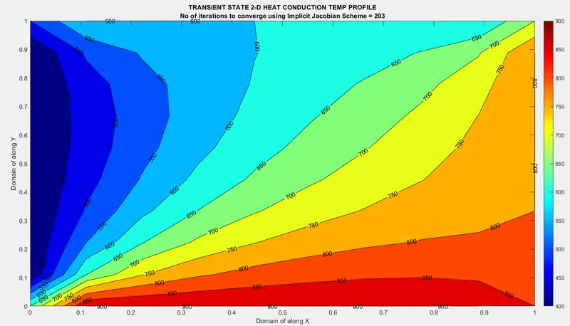
(2) Implicit Scheme (Gauss-Seidal)
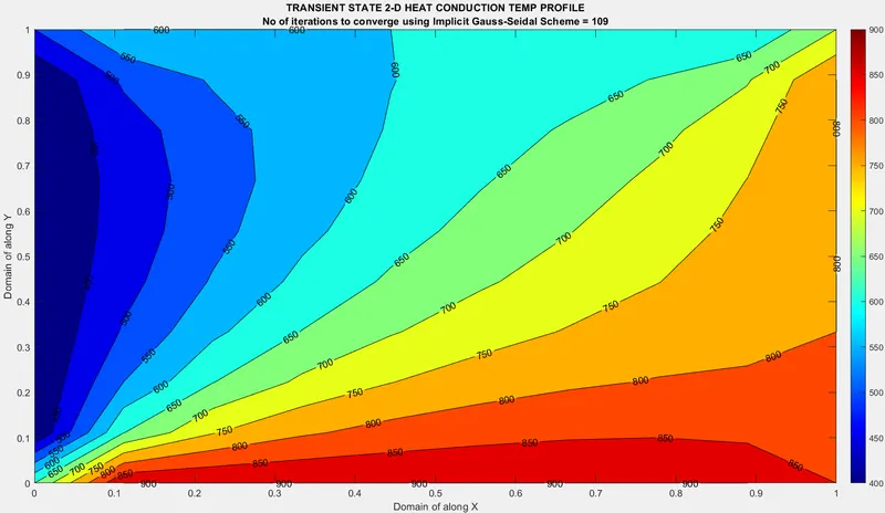
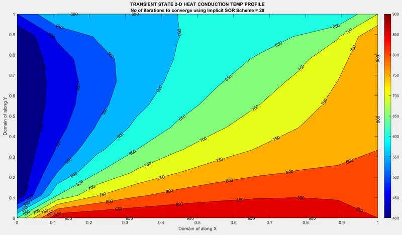
(3) Implicit Scheme (Successive Over Relaxation) for omega = 1.5
Conclusion :
|
||||||||||||||||||||||||||||||||||
- Iterative Methods with continuous updation of values over step size tend to converge at the earliest with least computation Time
- SOR method involves dependency on the limit of Relaxation factor for converging the solution. An ideal SOR method involves omega ranging from 1 to 1.5
For omega = 2.5
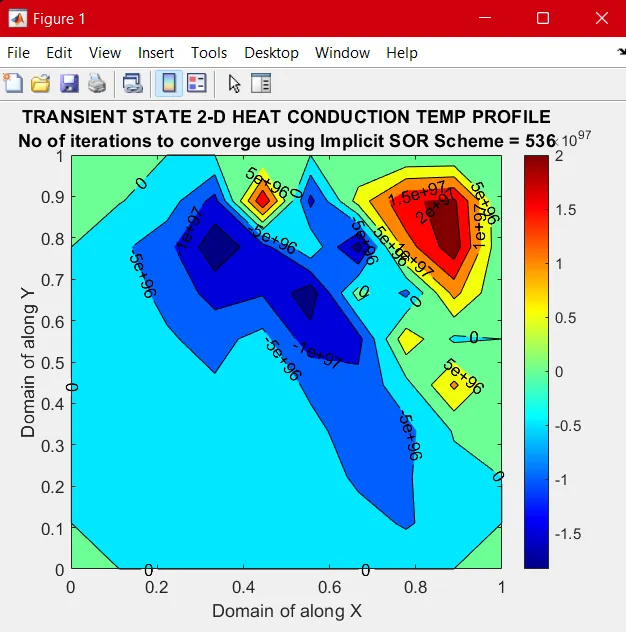
Oscillations over the solution and iteration continues greater than 4000 nos.