Simulating Fluid Sloshing effect inside a Gear-box

Part - I

1) Geometry setup :

prepare -> volume extract -> select the fluid volume by selecting all the edges of 4 openings -> Ok

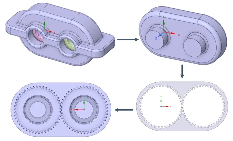
• Hide the solid volume and the left will be fluid volume which we generated.
• Now we have to split this body into half to extract the 2D geometry right in the middle plane.
• First create planes by selecting plane in design and click on origin ,which creates 2 planes X,Y and Z planes.
• We use the split body command in spaceclaim which is under design to split the geometry it into two parts by selecting the geometry and plane and delete the other part.
• Now we can see the interior sectional view.Now if you select the top part of the remaining geometry you can see the yellow top face part,which is what we want .Inorder to extract that area we need to select that face and copy and open new design and then paste it and save it.
• Now reset the setup and import the 2D saved geometry and open the meshing module.
• The below image is the final 2D geometry that we simulate.

Meshing :

• Go to Mesh > Right Click> Methods > All Triangles

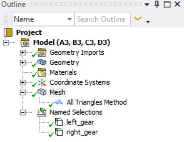
• Mesh each and every single edge left in the gear element

• Go to Named Selections and name left and right gear

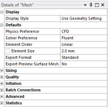
• Element Size > 2mm ----- Proximity Curvature - ON
• 

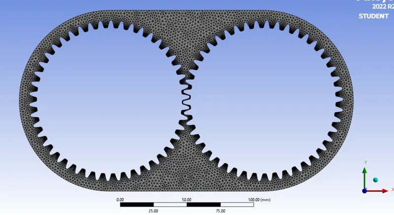
• Total No of Elements = 17089

Solving :

Solver

• Pressure Based
• Transient
• With gravity in Y

Materials

• Air ----------------ρ">ρ� = 1.225 kgm3">kgm3���3 ; Viscosity = 1.7894e-05 kgms">kgms����
• Engine Oil---------ρ">ρ� = 889 kgm3">kgm3���3 ; Viscosity = 1.06 kgms">kgms����
• n-heptane---------ρ">ρ� = 684 kgm3">kgm3���3 ; Viscosity = 0.000409 kgms">kgms����

Multiphase

Models

• VOF Method
• Implicit Formulation

Phases

• Name the material phases
• Choose appropriate phase material

User defined Function (UDF)

• Below codes give the rtational angular velocity for both left and right gear
• Go to user defined > Click on Functions > Compiled > Go to ADD > Choose the .c file > Then Build and Load

#include "udf.h"

DEFINE_CG_MOTION(right_motion, dt, vel, omega, time, dtime)
{
	vel[0] = 0.0;
	vel[1] = 0.0;
	vel[2] = 0.0;

	omega[0] = 0.0;
	omega[1] = 0.0;
	omega[2] = 2.0e2; /* [rad/s]*/
}
DEFINE_CG_MOTION(left_motion, dt, vel, omega, time, dtime)
{
	vel[0] = 0.0;
	vel[1] = 0.0;
	vel[2] = 0.0;

	omega[0] = 0.0;
	omega[1] = 0.0;
	omega[2] = -2.0e2; /* [rad/s]*/
}

Marking Cells

• Defining the regions where the fluid is present for 20% and 30% imeersion respectively
• For this, go to Spaceclaim and mark rectangular boxes to he geometry to identify the 20mm and 30mm marks on the geometry

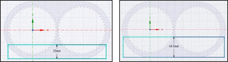
20% Immersion Co-ordinates :

• Xmin">Xmin�min = -0.0580m
• Xmax">Xmax�max = 0.1730m
• Ymin">Ymin�min = -0.0345m
• Ymax">Ymax�max = -0.0675m

30% Immersion Co-ordinates :

• Xmin">Xmin�min = -0.0650m
• Xmax">Xmax�max = 0.1800m
• Ymin">Ymin�min = -0.018m
• Ymax">Ymax�max = -0.0675m

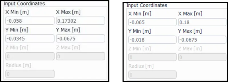
Dynamic Mesh

• Domain > Mesh Models > Dynamic Meshing
• Enable Dynamic Meshing

Mesh Methods

• Enable Smoothing
• Enable Layering
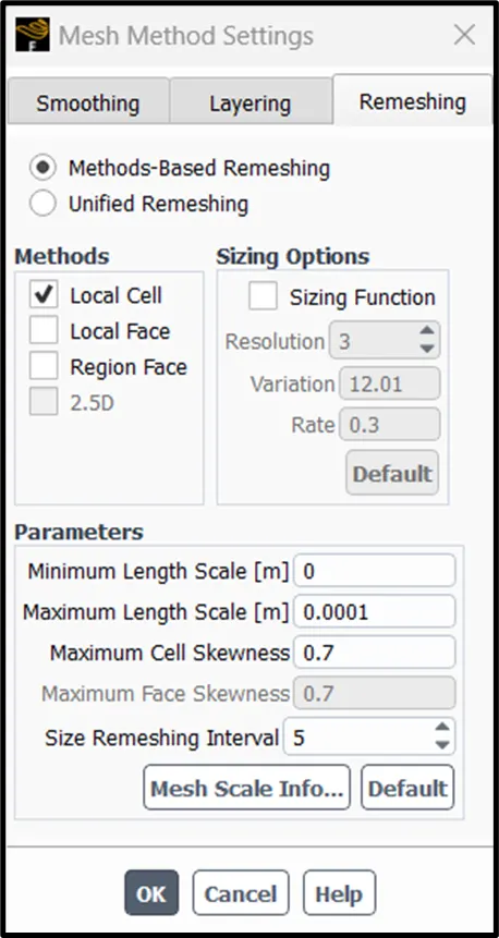
• Enable Remeshing
• Settings > Remeshing > Methods - based Remeshing > add values given in fig below

Dynamic Mesh Zones

• Go to Create/Edit
• Zone Names => Left Gear ---CG - x=[0m], y =[0m]

=> Right Gear--CG- x=[0.115m], y =[0m]

• Check for Motion of these gears by Display Zone Motion

Initialization

• Hybrid Intialization
• Patching for region of fluid
• Setting up Contous for Volume of Fluid

Time-Step Calculation:

• Angular Velocity - ω">ω� = 200rad/s
• ω=2⋅π⋅N60">ω=2⋅π⋅N60�=2⋅�⋅�60

where N - no of revolutions / second

∴">∴∴ N = 31.8 revolutions / second

• Time taken for the gear to rotate once = 1/31.8 = 0.031s for one rotation

For our simulation, we need a minimum of two rotations to capture, hence

• Total Flow Time = 0.031*2 = 0.062s

• Total Flow Time = No of Time Steps x Time Step Size

• Keeping the time step size to be well beyond 1e-4 to avoid negative volume generation or numerical diffusion, hence No of Time steps for our calculation will be 620

• Total Flow Time = 0.062s
• Time step size = 1e-4s
• No of time Steps = 650

Solutions

Case I : 20% Immersion - Engine Oil

https://youtu.be/XGj0Ab6R3tk

Case II : 20% Immersion - n-heptane(liquid)

https://youtu.be/LNAubK-hxlU

Case III : 30% Immersion - Engine Oil

https://youtu.be/tnUNFdPgfMA

Case IV : 30% Immersion - n-heptane(liquid)

https://youtu.be/CGtvhe4Gcvg

Part - II

Dynamic Meshing

• It is used to model flows where the shape of the domain is changing with time due to motion on the domain boundaries
• The moving-mesh provides a capability of tackling flow simulations where the domain shape changes during the simulation.
• In such cases, the computational mesh needs to adapt to the time-varying shape of the domain and preserve its validity and quality.
• The mesh motion solver support which calculates the internal point motion based on the prescribed motion of the boundary.

Types and Character of Mesh Motion

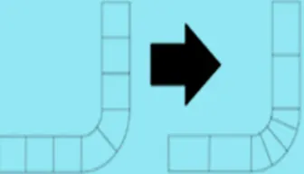
• H- Method - It involves automatic refinement of the spatial mesh based on error estimates or error indicators.

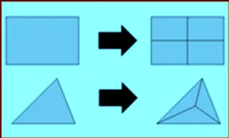
• R-Method - It is also known as the Moving mesh method. It relocates grid points in the mesh in way where the gradient of property in increasing rapidly in that region

Examples where Dynamic Meshing is used :

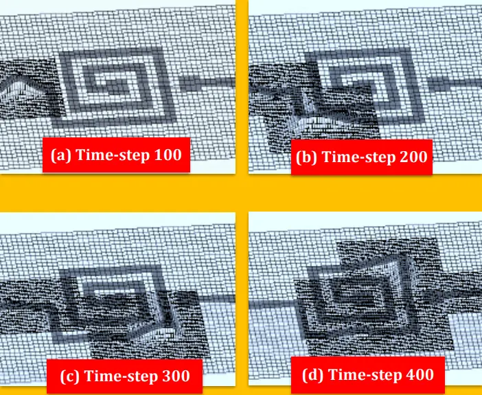
1. Wavefront Tracking for a spiral inductor - Dynamically Adaptive Mesh Refinement (DAMR)

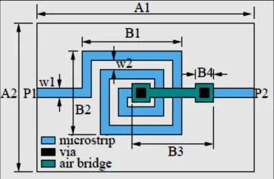
• Above image is a spiral inductor with ports P1 & P2.
• Due to field flow through this spiral inductor, an electric wave front is created vertically into the screen.
• Due to its high speed motion, capturing such rapidly changing boundary physics can only be done in Dynamic Adaptive Mesh Refinement technique.
• Due to highly resonant nature of the spiral inductor, which requires the use of a significant number of time steps for the extraction of parameters, AMR significantly reduces the usage of such high number of time steps
• Child meshes converges to zero over time, implying that only the root mesh is still present at a late stage of the code
• Hence, no spatial or temporal interpolation operations, which are the primary
  sources of instabilities in adaptive mesh codes
• This is an additional advantage of using a dynamically adaptive instead of a statically adaptive mesh in time-domain simulations

2. Sliding Mesh Interface for Vertical Axis Wind Turbine (VAWT)

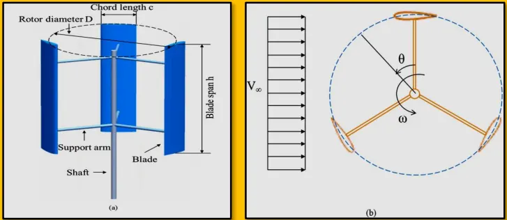
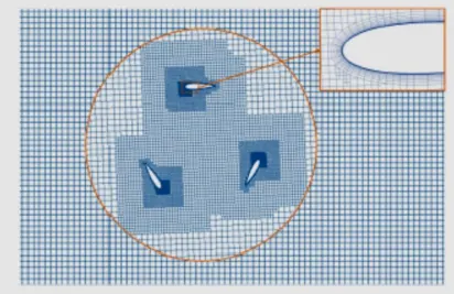
• domain can be divided into an outer zone and a rotating inner zone
• the center of the inner zone is situated at 5 rotor diameters downstream of the inlet boundary and 15 rotor diameters upstream of the outlet
  boundary, which can allow for sufficient space for the wake generation
• The width of the outer zone is 10 times the rotor diameter while its height is 3 times the blade span
• For the inner zone, its diameter is 2 times the rotor diameter and its height is 1.5 times the blade span

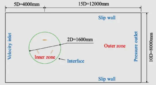
• A uniform velocity profile is set as the inlet condition and the outlet boundary is considered as pressure outlet with zero relative pressure
• The slip wall condition is assigned to the remaining boundaries of the outer zone
• No-slip wall condition is assigned to blade surfaces

Fluid Sloshing Effect

• It is the movement of the liquid inside another object due to an external forcing onto the object or due to internal forcing such as a gear.
• The liquid must have a free surface to constitute a sloshing problem, where the dynamics of the liquid can interact with the container to alter the system dynamics significantly.
• Sloshing has negative effects in the case of a container containing liquid.
• It can result in structural damage to the walls of the object due to the hammering effect of the liquid in repeated intervals.
• Sloshing can be hazardous during the transport of reacting chemical liquids.
• To prevent sloshing in containers, Baffles are used. Baffles are essentially walls that reduce the effective free surface elevation attained by the liquid during sloshing. It is also experimentally observed that with an increase in the viscosity of the fluid, the damping effect on the slosh increases.

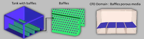
credits: @LearnCAx

In the case of a gearbox, the liquid sloshing has a positive effect. It helps in the complete lubrication of the gear tooth. The lubricant is able to find itself in each and every tooth of the gears.

What is the use of UDF?

• Customize boundary conditions
• Material property definitions
• Adjust computed values on a once-per-iteration basis.
• Enhance post-processing

Common errors that occurred in the simulation

Negative Cell Volume detection

• If Displacement of boundary > Local Grid size it can give rise to Negative Cell Volume detection
• This basically means that the edge of the cell can penetrate the vertex or the edge of the other cell
• This brings down the skewness quality of cells

Dynamic mesh failed

• Mesh distortion is bound to happen for dynamic meshes
• Continuous resizing and remeshing of these distorted meshes can avoid getting this error
• Hence usage of Remesh can give us the control to input remeshed cell sizes of minimm and max capture lengths