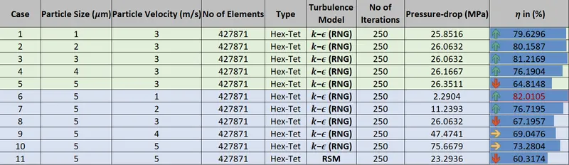
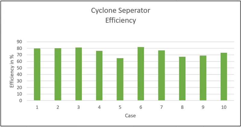
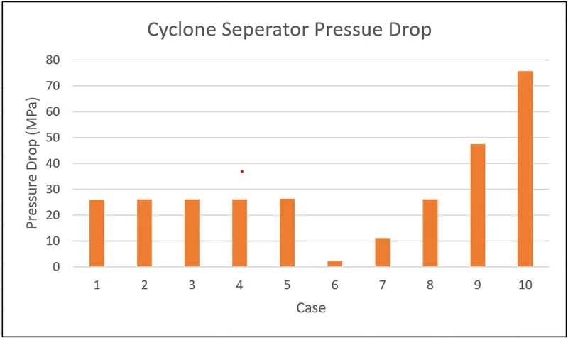
Week 8 - Simulating Cyclone separator with Discrete Phase Modelling
Empirical models
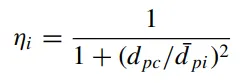
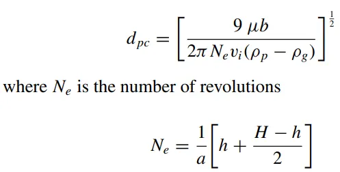
1) Iozia and Leith model - This model was developed based on force balance. In this model, since the particle undergoes vortex flow, two main forces are considered - i.e, centrifugal force and flow resistance.
The collection efficiency(ηi) of particle diameter(dpi) is given as
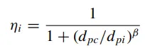
where

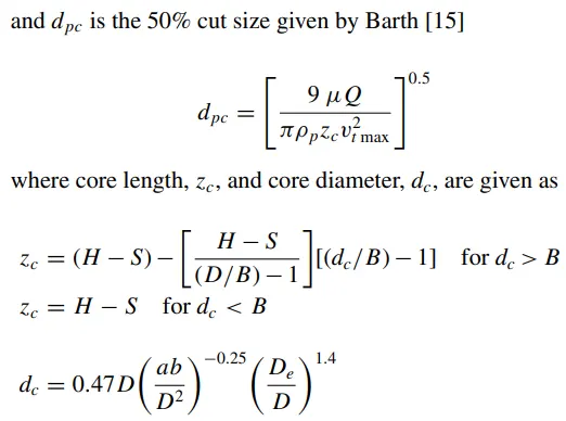
2) Li and Wang model - This model includes particle bounce or re-entrainment and turbulent diffusion at the cyclone wall. In this model, 2D analytical expression of particle distribution in the cyclone is given as
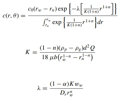
where
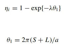
3) Koch and Licht model - This model includes the inherently turbulent nature of cyclones and the distribution of gas residence times within the cyclone.
A force balance and an equation on the particles collection yields the grade efficiency (ηi) as
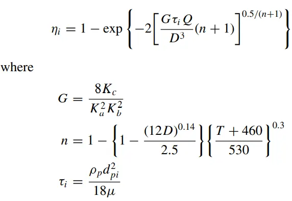
4) Lapple model - This model was developed based on force balance without considering the flow resistance. Lapple assumed that a particle entering the cyclone is evenly distributed across the inlet opening.
The efficiency of collection of any size of particle is given by -
Analysis on a given cyclone separator model by varying the particle diameter from 1 μm to 5 μm
> Extract volume from Volume Extract by selecting edge selection
> Suppress the physics for which the volume is not required for simulation
> Then enter meshing
> Choose Mesh > Right click > Select Method > Body Fitted Cartesian
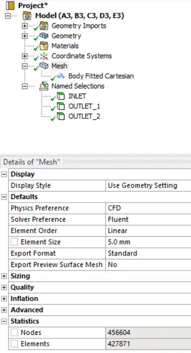
> Let element size be 5mm
> Generate Mesh
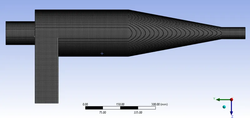
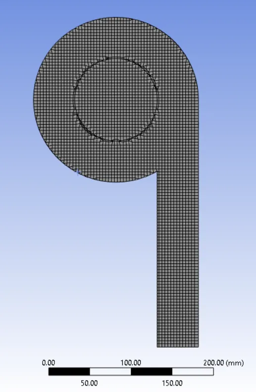
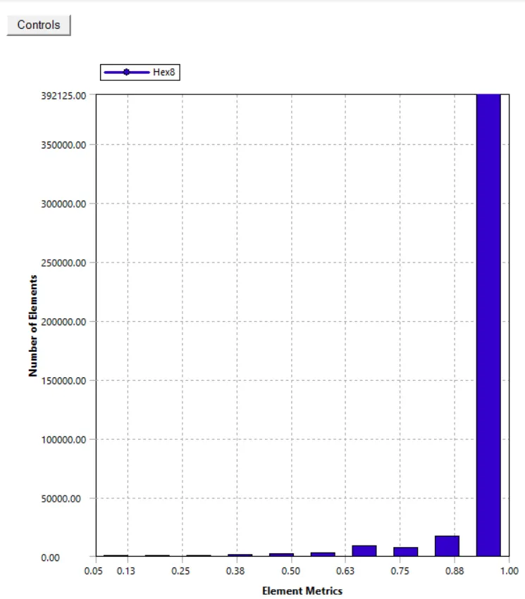
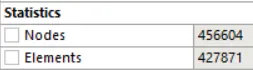
Analse mesh stats & quality
> Go to Fluent Solver & enable gravity in y direction
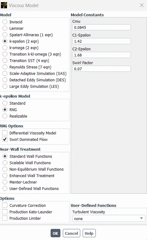
> Choose turbulence model for k-e (RNG) > swirl dominant flow
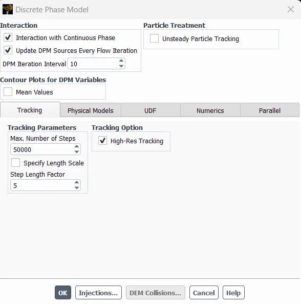
> Set up Discrete Phase Model
> Setup injections settngs
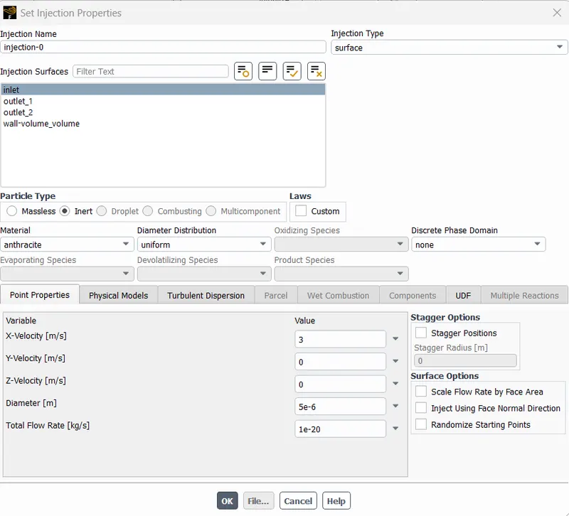
> Set BC's for the above
Inlet : X - 3m/s & DPM - Reflect
Outlet-1: p = 0 & DPM - Escape
Outlet-2: p = 0 & DPM - Trap
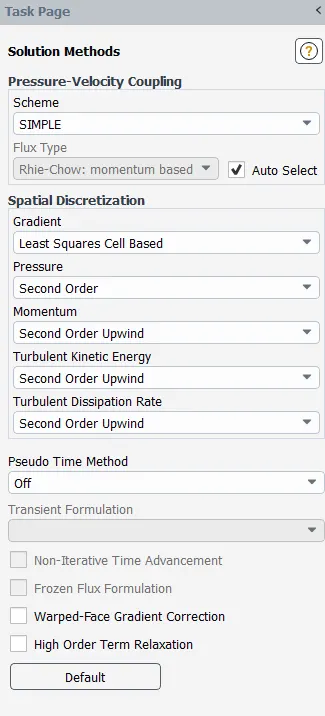
Solution Scheme:
P-V Coupling:
* SIMPLE Scheme
Spatial Discretization:
*Gradient: Least Square Cell based
*Pressure: II Order
*Momentum: II Order Upwind
*Turbulent Kinetic Energy: II Order Upwind
*Turbulent Dissipation Rate: II Order Upwind
> Report definitions > Check for static pressure at Inlet & Outlet1 for calculation pressure drop
> Standard Intialize the solution from Input
> After simulations > Export the particle history data to some file for post processing purpose
Efficiency is calculated by
`eta =`(No of particles trapped) / (No of partcles tracked)
Results:
Case:1-
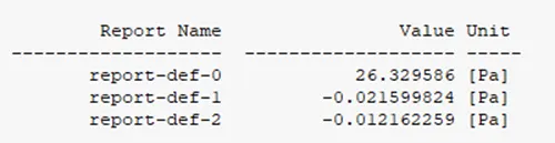
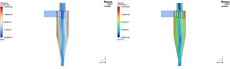
Residuals & Pressure plot @ Inlet & outlets:
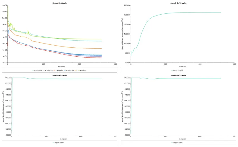
pressure drop:
Efficiency:

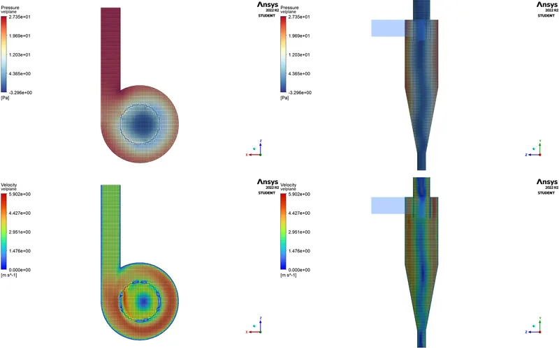
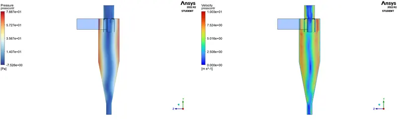
Pressure & Velocty contours:
Case:2-
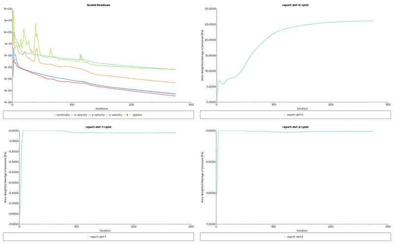
Residuals & Pressure plot @ Inlet & outlets:
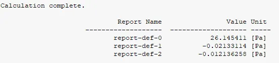
pressure drop:
Efficiency:

Pressure & Velocty contours:
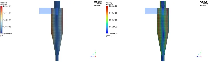
Case:3-
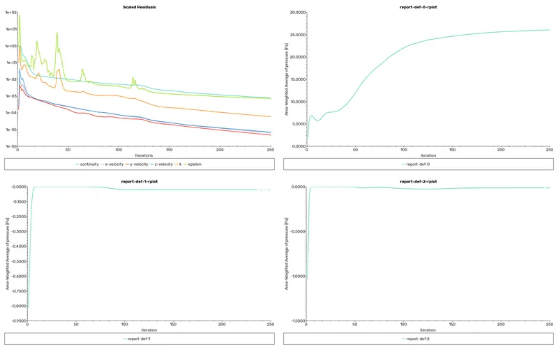
Residuals & Pressure plot @ Inlet & outlets:
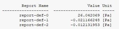
pressure drop:
Efficiency:

Pressure & Velocty contours:
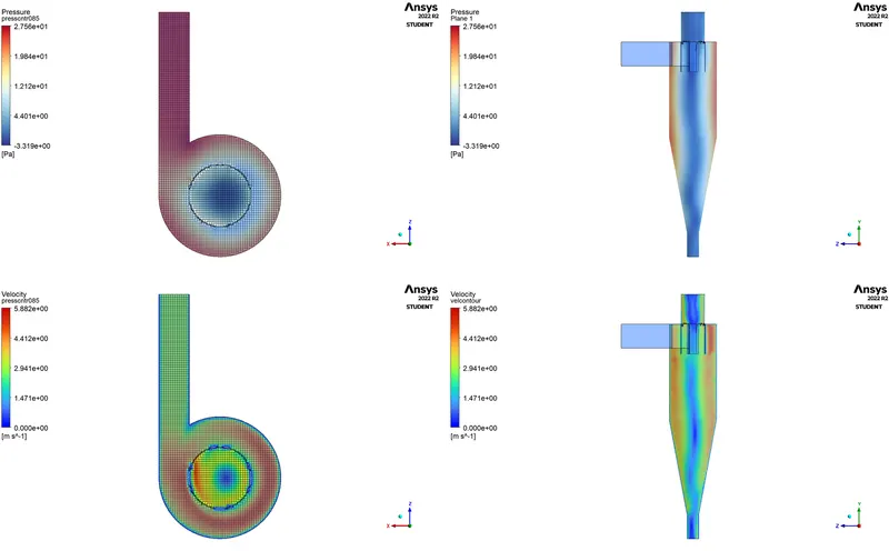
Case:4-
Residuals & Pressure plot @ Inlet & outlets:
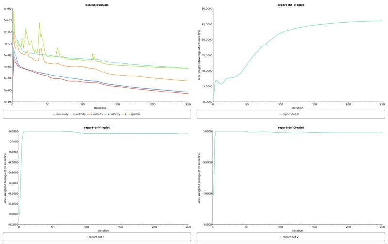
pressure drop:
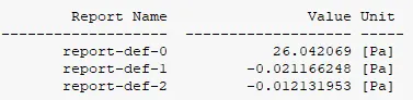
Efficiency:

Pressure & Velocty contours:
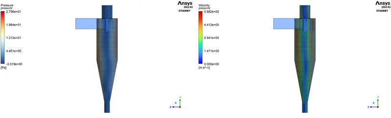
Case:5-
Residuals & Pressure plot @ Inlet & outlets:
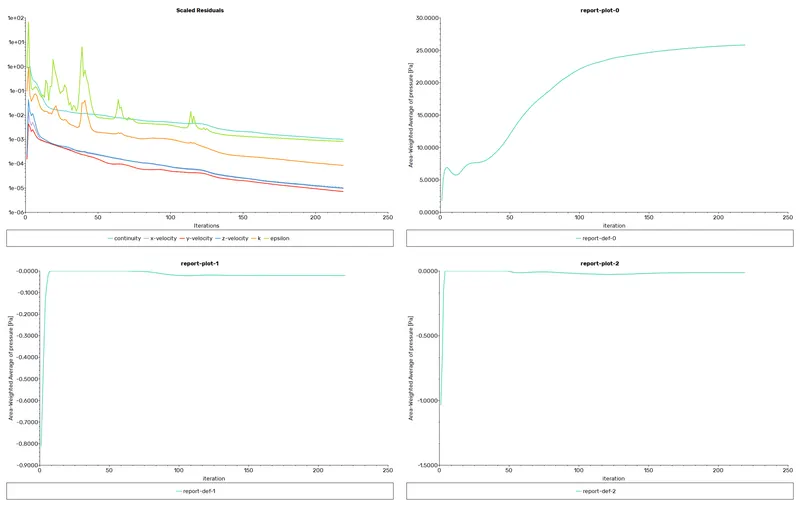
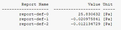
pressure drop:
Efficiency:

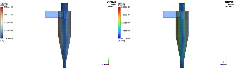
Pressure & Velocty contours:
Case:6-
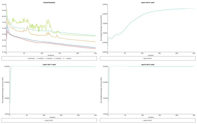
Residuals & Pressure plot @ Inlet & outlets:
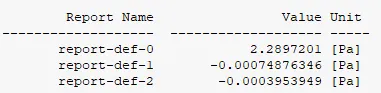
pressure drop:
Efficiency:

Pressure & Velocty contours:
Case:7-
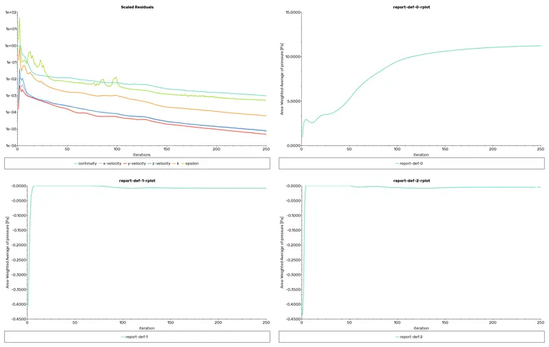
Residuals & Pressure plot @ Inlet & outlets:
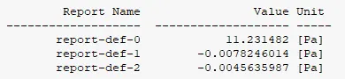
pressure drop:
Efficiency:

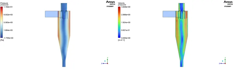
Pressure & Velocty contours:
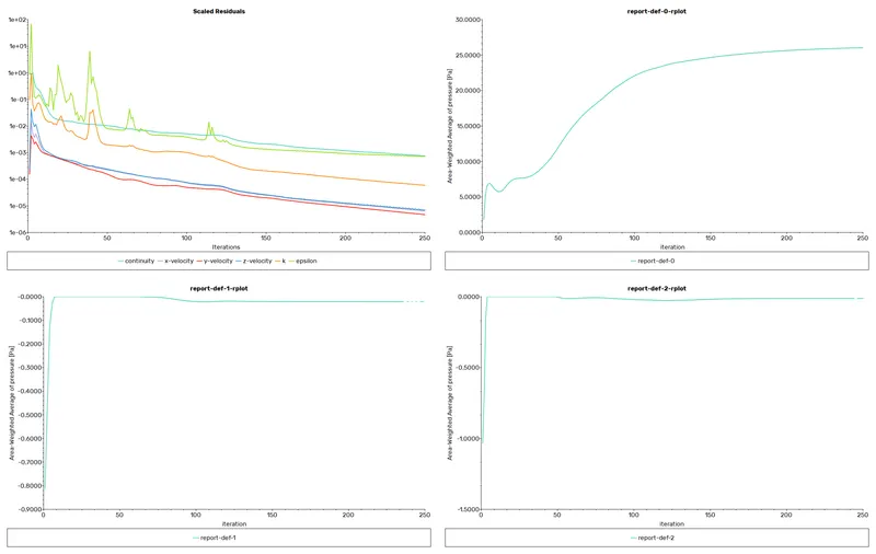
Case:8-
Residuals & Pressure plot @ Inlet & outlets:
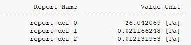
pressure drop:
Efficiency:

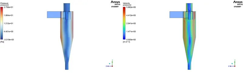
Pressure & Velocty contours:
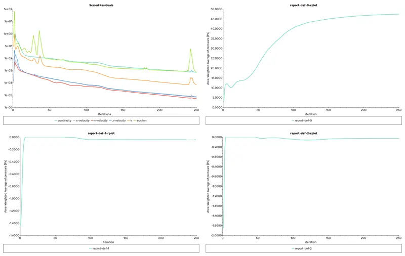
Case:9-
Residuals & Pressure plot @ Inlet & outlets:
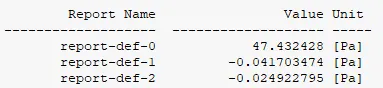
pressure drop:
Efficiency:

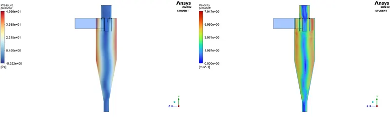
Pressure & Velocty contours:
Case:10-
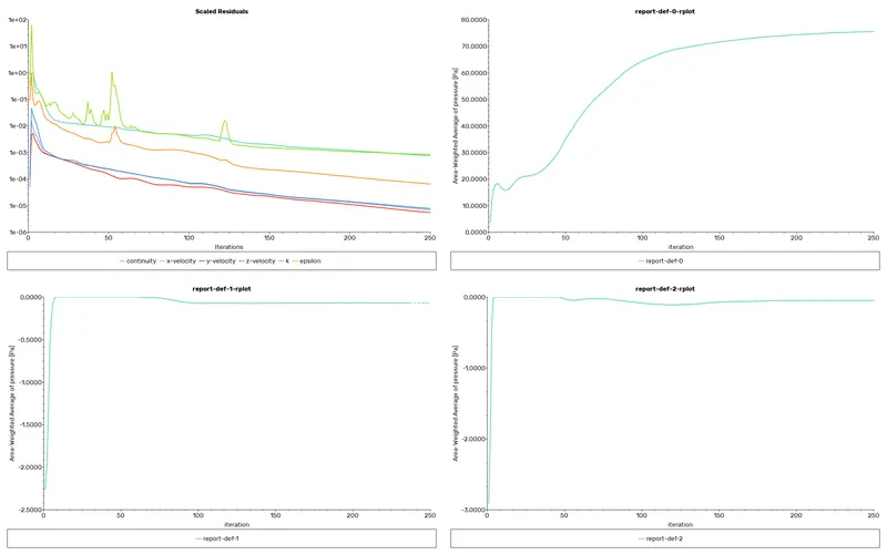
Residuals & Pressure plot @ Inlet & outlets:
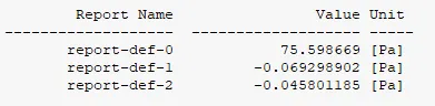
pressure drop:
Efficiency:

Pressure & Velocty contours:
Final Results & Calculations for comparison of Efficiency: