Week 3 - Solving second order ODEs
Simple Harmonic Oscillation of Simple Pendulum
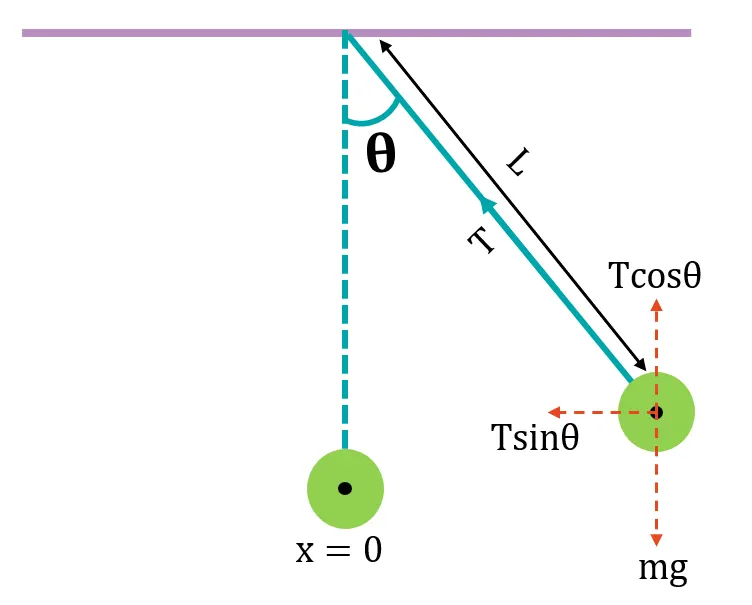
Discretizing the forces acting on a simple pendulum by drawing the force body diagram (FBD) gives us a better understanding of the approximations and assumptions to be made to calculate damp free oscillating motion of Simple pendulum.
Let
L be the length of the string,
m be the mass of the bob
`θ` be the angle made by the bob against the vertical y axis
T be the tension on the string
Now calculating the forces on X Direction:
x: `m ((d^2 x)/(dt^2 )) =-T_θ sinθ- T_θ x/l`
y: `m ((d^2 y)/(dt^2 )) =T_θ cosθ- mg`
Therefore `T_θ = mg`
Approximations made:
i) Small Angle approximations
When θ<<<<1 (radians), then the angle is considered to be small angle.
Consequence 1 : cosθ ≈ 1
Consequence 2 : Distance excursion y <<<< Distance excursion in x,
hence acceleration in y is ≈ 0
Therefore
`m ((d^2 x)/(dt^2 )) + mg x/l=0`
Dividing the equation throughout by m,
`((d^2 x)/(dt^2 )) + x g/l=0`
This above equation is the Simple Harmonic Oscillation equation without dampness being considered.
Now considering dampness as a factor while oscillating the equation become:
`(d^2 θ)/(dt^(2 ) )+ b/m dθ/dt+ g/l sinθ=0`
Transforming the second order ODE to first order ODE:
Let `θ`= `θ_1`
therefore
`d/dt(θ) = (dθ_1)/dt = θ_2`
`(d^2 θ)/(dt^2 ) = d/dt((dθ_1)/dt)` = `d/dt(θ_2)`
`(d^2 θ)/(dt^2 )= (dθ_2)/dt = (-b)/m θ_2- l/g sinθ_1`
and
`d/dt (θ_1)` = `θ_2`
Creating a matrix form of the above two equations, we get
`d/dt[[θ_1],[θ_2]] = [[θ_2], [(-b)/m θ_2- l/g sinθ_1]]`
now we can combine the solution vector as below:
`d/dt[θ] = [[θ_2], [(-b)/m θ_2- l/g sinθ_1]]`
From the above method let us solve for theta, using the ODE function in MatLab
MatLab Code for solving θ in a second order ODE:
Initial Conditions & Data considered for solving the below equation
`(d^2 θ)/(dt^(2 ) )+ b/m dθ/dt+ g/l sinθ=0`
Damping coefficient (b) = 0.05;
Mass of the bob = 1 kg;
Acceleration due to gravity = 9.81 m/`s^2`;
Length of the string = 1m
close all
clear all
clc

% Given Data
b = 0.05;
m = 1;
g = 9.81;
l = 1;

% initial conditions...
initial_conditions = [0;3];

% Limits of Integration
t_span = linspace(0,20,500);

% Solving using ODE45.....

[t,results] = ode45(@(t,theta) ode_fun(t,theta,b,g,l,m),t_span,initial_conditions);

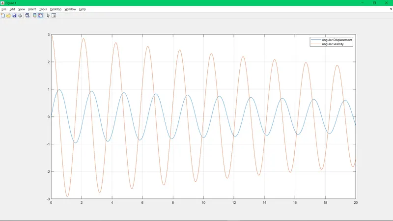
% Plotting the Output sinusoid curves for Velocity & displacement....
figure(1)
plot(t,results(:,1));
hold on
plot(t,results(:,2));
grid on
legend('Angular Displacement','Angular velocity')

% Creating an animation file for SHM oscillation of Bob...
angular_displacement = results(:,1);
ct = 1;
for i = 1:length(angular_displacement)
    angular_displacement1 = results(i,1);

    % Input of known conditions
    x0 = 0;
    y0 = 0;

    x1 = l*sin(angular_displacement1);
    y1 = -l*cos(angular_displacement1);

    figure(2)

    % Plotting the horizontal support for Pendulum....
    plot([-1 1],[0,0],'color','g','linewidth',3);
    hold on

    % Plotting the line for the massless string....
    line([x0 x1],[y0 y1]);
    hold on

    % Plotting the motion of Bob...
    plot(x1,y1,'Marker','o','Markersize',30,'Markerfacecolor','k');
    hold off
    grid on
    axis ([-2 2 -2 2])
   % pause(0.00000003)
    M(ct) = getframe(gcf);
   % pause(0.00000003)
    ct = ct+1;
end

% Creating a movie of variable M which contains all frames
movie(M);

% Writing the video
videofile = VideoWriter('SHM_Simulation.avi');

open(videofile)

writeVideo(videofile,M)

close(videofile)
Coding explaination for plotting & simulation:
1. Giving the initial conditions for `d/dt[[θ_1],[θ_2]] = [[θ_2], [(-b)/m θ_2- l/g sinθ_1]]` where angular displacement `theta_1`= 0 radians & angular frequency`theta_2`= 4 radians/s.
2. Since we are using the "ode45" function to solve for the second order ODE, we have to give the specific integrating limits which is time in this case. Hence time is given as a variable which takes 500 values between 1 to 20 seconds.
3. Following the syntax for "ode45", the results are calculated for both time and functions we have given as an input since we need to calculate Angular displacement as well as Angular velocity of the bob.
Then followed on the right end of the equation, "ode45" function takes three inputs where we need to seperately create a function to solve for angular displacement and then input the independent variables using an anonymous function "@" , input the t_span array & then mention the array vector of initial condition given above.
Creating the function to solve for Solution Matrix:
function solution_matrix = ode_fun(t,theta,b,g,l,m)
theta1 = theta(1);
theta2 = theta(2);
dtheta1_dt = theta2;
dtheta2_dt = -(b/m)*theta2 - (g/l)*sin(theta1);
solution_matrix = [dtheta1_dt; dtheta2_dt];
end
4. `d/dt[[θ_1],[θ_2]] = [[θ_2], [(-b)/m θ_2- l/g sinθ_1]]`
Comparing the solution matrix vector we can create a function which is dependent on b,g,l,m,t & define `θ_1 & θ_2`as above.
Then from the above equation , equate the values of the solution matrix & define the final solution matrix as above.
5. Plotting the sinusoid curves for Angular Displacement & Velocity:
"plot" command can be utilized and calling the angular displacemnt seperately by using results(:,1), here 1 represents the 1st column of the result which is Angular Displacement & similarly 2 represents Velocity
6. Animation of the Pendulum:
"for" loop can be utilized to calculate the positions of the bob over numerous variations of angular displacement. Then input the co-ordinates for string & the bob to create a motion.
Now to create a support for the Pendulum, plot a line of 2 m in magnitude & plot a line for string which is dependent on the values of X0, Y0 & X1, Y1. After this the motion of bob could be plotted which is a function of the co-ordinates X1 & Y1. A Marker command could be used to create a "o" size shape of specific marker size.
Store these frames by collecting these frames into a variable called M. Then we can use this to write the videofile and then create a movie of AVI format.
Errors commited while coding:
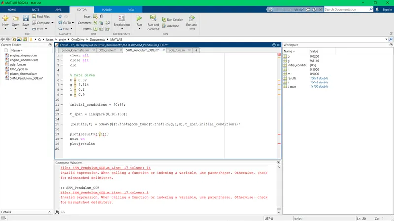
1. Inorder to plot the values for Angular displacement seperately, we have to use a colon operator to perform this operation, instead an error was commited by using a semicolon operator
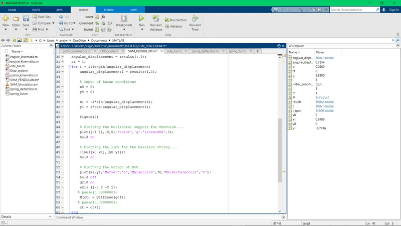
2. While discretizing the components of bob, an error was made where the reference axis was taken in the opposite direction for y axis. This created the motion to swing the bob in the positive y axis.
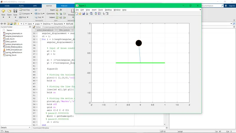
Animation of the bob: (Youtube Link)
https://youtu.be/HDhRGHedRGs