Linear Convection for varying time steps and understanding significance of CFL number for solution stability

To calculate `U_( f i n a l)` & X of Linear Convection equation for set of time steps & plot `U_( f i n a l)` vs X

Motivation to understand Time & space marching problems:

Linear Convection part of the Navier stokes equation is given by

Indexing for 'u' to characterize space & time marching elements :

where

n is the Time index

x is the space index

Let us consider a square wave form with nodes & specific data to apply time & space marching approach

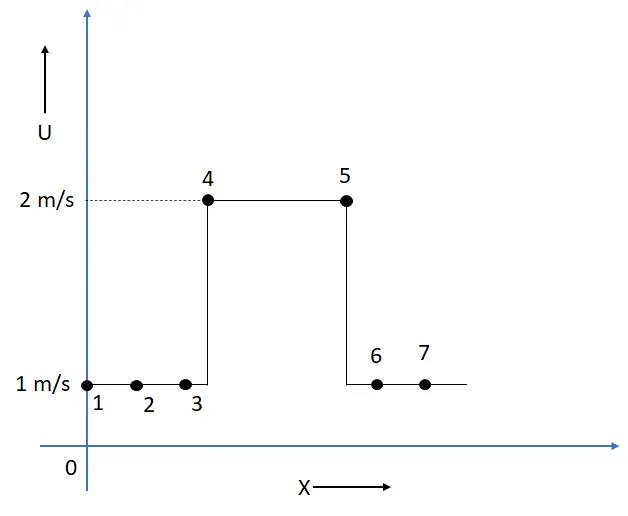
Applying forward differencing of 2nd order accuracy to time derivative term & backward differencing of 2nd order accuracy to spatial derivative term

Given Data & problem to be solved :

Write a function that accepts the time step as an argument and solves the same problem. You will compare the effect of the time step on the numerical solution.

1. Number of nodes, n = 80

2. Time step , dt = 1e-4, 1e-3, 1e-2, and 1e-1

3. Simulation run time , t = 0.4 seconds.

Main code to calculate X & U for set of dt :

%% Approximating U_final with variable time steps

clear all
close all
clc

% Input Data
L = 1;                       % Length of domain
n = 80;                      % No of grid points
c = 1;                       % Constant convection cooefficient
dt = [1e-4,1e-3,1e-2,1e-1]; % Time step 
t = 0.4;                     % Integration time

% Calculating Run time for each dt for output of U & X using Tic & toc 

tic
[x1,u1] = linear_convection_var_timestep(L,n,c,t,dt(1));
run_time1 = toc;

tic
[x2,u2] = linear_convection_var_timestep(L,n,c,t,dt(2));
run_time2 = toc;

tic
[x3,u3] = linear_convection_var_timestep(L,n,c,t,dt(3));
run_time3 = toc;

tic
[x4,u4] = linear_convection_var_timestep(L,n,c,t,dt(4));
run_time4 = toc;

% Plotting all output from different timesteps of U vs X in single figure
figure(1)
plot(x1,u1,'color','k','linewidth',1)
hold on
plot(x2,u2,'color','g','linewidth',1)
hold on
plot(x3,u3,'color','r','linewidth',1)
hold on
plot(x4,u4,'color','b','linewidth',1)
hold on
grid on
axis([0 1 0 2.2]);
xlabel('X')
ylabel('U Final')
legend('Time Step 1 = 1e-4', 'Time Step 2 = 1e-3','Time Step 3 = 1e-2','Time Step 4 = 1e-1','location','Northeast')
title('Final Velocity profile for varying Time Steps') 

% Plotting  Run Time vs Time step on Bar graph
figure(2)
Time_Step = categorical({'1e-4','1e-3','1e-2','1e-1'});
Run_Time = [run_time1 ,run_time2, run_time3, run_time4];
bar(Time_Step,Run_Time);
grid on
xlabel('dt (s)')
ylabel('Run Time (s)')
title('Run time vs Time step')

Function code to calculate X & U :

%% Function to calculate x,u_final with variation in time steps & other parameters

function [x,u] = linear_convection_var_timestep(L,n,c,t,dt)
           

           % Calculating Grid parameters
              x  = linspace(0,L,n); % Meshing for length L
              dx = x(2)-x(1);       % Grid Size
           
           % Calculation no of time steps
              nt = t/dt;
           % Given Data for starting & ending points of change in Velocity
         n_start = 0.1;
          n_stop = 0.3;
                  
           
           % Assuming values of x are in A.P with difference dx
           % n_start = 0 + (f_start - 1)*dx (nth term of an AP)
           % n_stop  = 0 + (f_stop - 1)*dx 
                 f_start = round((n_start/dx)+1);
                 f_stop  = round(n_stop/dx)+1;
                 
           % Initializing U array & setting BCs
                       u = 1*ones(1,n);
       u(f_start:f_stop) = 2;
       
           % Applying Boundary Conditions 
                    u(1) = 1;
                    uold = u;
                 
                     
           % Time Loop
                  for i  = 1:nt
                
           % Space Loop    
                    for j = 2:n
                     u(j) = uold(j) - (c*(dt/dx)*(uold(j) - uold(j-1)));
                    end
                
           % Update old Velocities
                     uold = u;
                                
                  end
end

Main Code Explaination :

• Defining input parameters for L, n, c, dt & t
• Tic & toc are used to calculate simulation time for each time step
• Starting & ending points of change in velocity are also mentioned by n_start & n_stop
• A function is created with an input of L, n, c, n_start, n_stop, dt & nt and with X & U being output values
• Defining meshing for length 'L' of the domain with 'n' grid points
• Defining grid size by the difference between two consecutive mesh points
• Calculating starting & ending points of change in Velocity by using Arithmetic Progression method

Nth Term of AP :

n_start = 0 + (f_start - 1)*dx Initial Value is set to 0
n_stop = 0 + (f_stop - 1)*dx

• To avoid floats, rounding off is done by using 'round'
• Initialising U array by creating the array of Ones of 1 row & n colums
• Initialising the value of u at n_start & n_stop = 2 m/s
• Setting up the Boundary condition u(1) = 1 m/s
• Assigining U as 'uold' value & creating a duplicate called 'u_initial' for further plot reference which is also the same as U
• To perform 'nt' time steps of operation, a for loop is introduced with 'j' as a counter running through the length of 'nt'
• Calculating U final by implementing Forward differencing scheme for Time marching term & Backward diff scheme for Space Marching term

Observation 1 :

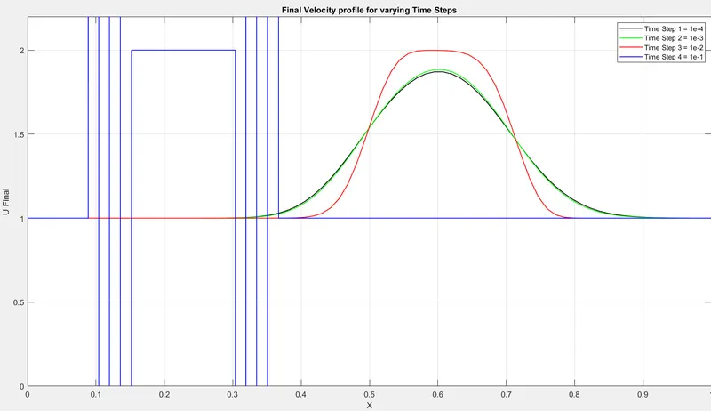
Observation 2 :

• Velocity Profile for dt = 1e-1

Velocity profile shows clear solution blowup and wiggles. (UNSTABLE SOLUTION)

• Velocity Profile for dt = 1e-2

STABLE SOLUTION with DIFFUSION DOMINANCE `=>` High Drop in Velocity

• Velocity Profile for dt = 1e-3

STABLE SOLUTION with mild DIFFUSION `=>` Less Drop in Velocity

• Velocity Profile for dt = 1e-4

STABLE SOLUTION with no DIFFUSION `=>` No Drop in Velocity

CFL Criterion for GDE :

Courant–Friedrichs–Lewy or CFL condition expresses that the distance that any information travels during the timestep length within the mesh must be lower than the distance between mesh elements. In other words, information from a given cell or mesh element must propagate only to its immediate neighbors.

`frac{delu}{delt} + c*frac{delu}{delx}=0`

Applying Upwind scheme for eqn (1)

`frac{U_i^(n+1) - U_i^(n)}{Deltat} +c*frac{U_i^(n) - U_(i+1)^(n)}{Deltax} = 0 =>(2)`

where c is the velocity magnitude

Performing Taylor's Series Expansion for eqn (2) :

On expanding eqn (2), numerical diffusion /num viscosity is introduced. As expected from a diffusion coefficient, the numerical diffusion coefficient must be positive, otherwise, the solution will grow indefinitely with respect to time, making the numerical scheme unstable.

where

`frac{c*Deltat}{Deltax}`is the Courant Number`

It follows from the numerical diffusion coefficient discussion, that for any explicit simple linear convection problem, the Courant number must be equal or smaller than 1, otherwise, the numerical viscosity would be negative

Effect of Change in Time step :

Observation 2 :

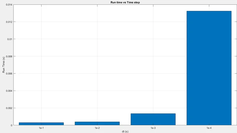
Calculating μnum">μnum for all time steps & Courant Number :

1. For dt = 1e-1

dx = 0.0126

c = 7.93 > 1, therefore artificial diffusion or numerical viscosity is negative

2. For dt = 1e-2

dx = 0.0126

c= 0.793 < 1 is a stable solution

μnum =(0.0063)⋅(1−0.0793)=0.0013m2s

3. For dt = 1e-3

dx = 0.0126

c=0.0793 < 1 is a stable solution

μnum =(0.0063)⋅(1−0.0793)=0.0058m2s

3. For dt = 1e-4

dx = 0.0126

c= 0.00793 < 1 is a stable solution

μnum=(0.0063)⋅(1−0.00793)=0.00625m2s

INTERPRATION :

For decrease in the time step, the solution converges accurately where dt from ie-2 to 1e-4 is showing positive Numerical Viscosity & for dt = 1e-4, the courant number > 1 which means that Numerical viscosity is negative which is physically insignificant which is an unstable solution