Week 2 - Flow over a Cylinder.
Week 2 - Flow over a Cylinder
Contents
1. Introduction to Vorticity
a) Viscosity (A messenger to introduce Vorticity)
b) Mechanism of Vortex Shedding
c) Vortex visibility regimes
2. Computational Domain
3. Meshing Methodologies
4. Physics & Solver Setup
5. Animation Methods
6. Results and Discussions
1. Introduction to Vortices
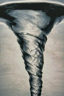
A vortex is a region in a fluid in which the flow revolves around an axis line, which may be straight or curved. Vortices are a major component of turbulent. The distribution of velocity,vorticity (the curl of the flow velocity), as well as the concept of circulation are used to characterise vortices. In most vortices, the fluid flow velocity is greatest next to its axis and decreases in inverse proportion to the distance from the axis.
a) Viscosity (A messenger to introduce Vorticity)
TO FIND THE PRESSURE BETWEEN 2 POINTS
CASE I : Inviscid & Irrotational Flows
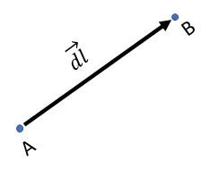
`vec(dl) = dx*hati + dy*hatj + dz*hatk`
Eulerian Equation of Motion in 3 dimensions
`-(delp)/(delx) + rho*b_x = rho*[frac(delu)(delt) + u*frac(delu)(delx) + v*frac(delu)(dely) + w*frac(delu)(delz)]` --------(1)
`-(delp)/(dely) + rho*b_y = rho*[frac(delv)(delt) + u*frac(delv)(delx) + v*frac(delv)(dely) + w*frac(delv)(delz)]` --------(2)
`-(delp)/(delz) + rho*b_z = rho*[frac(delw)(delt) + u*frac(delw)(delx) + v*frac(delw)(dely) + w*frac(delw)(delz)]`--------(3)
`-(delp)/(delx) + rho*b_x = rho*[frac(delu)(delt) + {vec V*(nablau)}]`---------(1*)
`-(delp)/(dely) + rho*b_y = rho*[frac(delv)(delt) + {vec V *(nablav)}]`---------(2*)
`-(delp)/(delz) + rho*b_z = rho*[frac(delw)(delt) + {vecV*(nablaw)}]`---------(3*)
Combining equation 1+2+3:
Simplifying RHS :
`[(delp)/(delx) + (delp)/(delx) + (delp)/(delz)] = dp`
Simplifying LHS :
TERM 1 :
`-rho*[frac(delvecV)(delt)*vec(dell)]`
TERM 2 :
`-rho*[(vecV*nablau)*dx + (vecV*nablav)*dy + (vecV*nablaz)*dz]`
TERM 3 :
`rho*[b_x*dx + b_y*dy + b_z*dz]`
Now for simplifying Term 2:
`-rho*[(vecV*nablau)*dx + (vecV*nablav)*dy + (vecV*nablaz)*dz]` = `-rho*[{(vecV*nabla)vecV}*vec(dl)]`
where
`(vecV*nabla)vecV` = `1/2 * [nabla(vecV*vecV) - vecVxx(nablaxxvecV)]`
Since vorticity is the curl of the velocity
`nablaxxvecV = vecOmega`
Therefore the rotationality of the depends on the value of `nablaxxvecV`
For Irrotational Flow :
`nablaxxvecV = 0`
i.e `[[hati,hatj,hatk],[frac(del)(delx),frac(del)(dely),frac(del)(delz)],[u,v,w]]` = 0
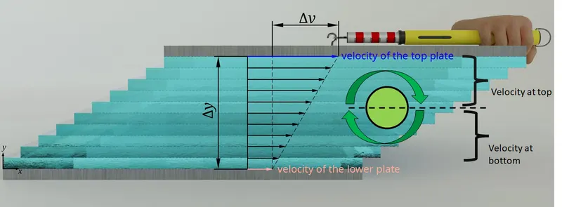
Considering the example of Flow between flat plates, wherein the velocity of top plate >>> velocity of bottom plate
If we consider the gradient of Velocity in Y direction, the velocity increases linearly from y = 0 to y=infinity; if a ball is placed in that medium, due to messenger called viscosity, the momentum difference between flow of fluid near to the bottom plate surface and flow of fluid at the centre and the top is felt by fluid and this is the reason why the force at top ball surface of the ball is greater than force at the bottom surface of the ball. Hence due to conservation of momentum difference, the ball would start rotating!
If fluid did not have viscosity as a messenger to propagate the momentum difference felt by different layers of fluid, then velocity throughtout the y axis of the distance between thne plates would reamin the same! Hence no momentum difference between layers of fluid and no rotationality!!
Hence Viscosity plays a mojor role for Vorticity in fluid.
NOTE :
An Inviscid Fluid is always Irrotational but an Irrotational Fluid is not always Inviscid !!
b) Mechanism of Vortex generation and shedding
Vortices are generated due to following reasons :
1. Presence of Viscosity : Due to Inviscid nature of fluid, boundary layer can grow and vary according to the profile of the geometry.
Bluff Nature of Body : If the body is blunt at the back of its geometry, vortices are expected to generate at the back of the bluff body, because bluff body can seperate the generating vortices into alternating vortices in upward and downward direction if the bluff body is divided into halves in y direction for discretized view.
Mechanism of Vortex Generation:
Understanding the Seperation Point
FRAME 1 :
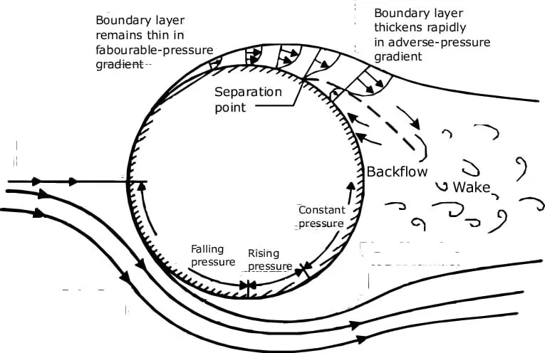
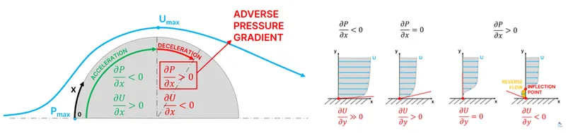
Considering air flowing from negative x axis towards positive x axis with origin of the axis begins from the surface of the cylinder. The first point of contact for air being the centre of the cylinder is a point where air nearly stops which was carrying a momentum before. This point is caled the Stagnation point where the pressure increases to maximum which we can denote it as `P_(max)`.
FRAME 2 :
Air after passing the stagnation with nearly 0 velocity, now accelerates from centre to the midpoint of the cylinder due to the favorable negative pressure gradient. Along the flow over the surface of cylinder, boundary layer is developed which is the layer where the velocity is comparably lower than the global free stream velocity, because this is the layer where frictional resistance due to viscosity comes into picture.
Velocity reaches a maximum value at the midpoint of the cylinder, with least thickness of boundary layer, indicating least resistances.
From here on this point, adverse effects of pressure gradients comes into picture. Till `U_(max)`, pressure gradient was the factor which drove to accelerate the flow over left half side of the cylinder. After `U_(max)` point, pressure now starts its journey in a positive pressure gradience. Pressure increases so bad that it actually starts resisting the flow, and flow begins to move in the reverse direction which is called Recirculation region
This leads to a point where forward directed flow and reverse directed flow meet at a point where velocity is 0, and pressure again is high which is called stagnation point for boundary layer seperation, which lifts the flow to move in the upward direction. This is the point of flow seperation from boundary layer.
FRAME 3 : What now happens after flow seperation?
Flow now follows the path of the shear layer. There are two sheared layers of two different dominant paths.
Vortices generated for Lower Reynolds number Flows (Stable Vortex Street)
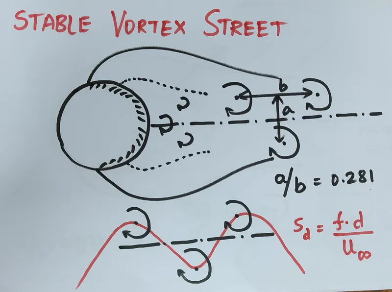
Two sheared layers are symmetrically developed forming very small vortices, this now develops to form alternative vortices on the top and bottom of the wake axis. This leaves a trail of vortices in the wake region generated in the same fashion called as Von-Karman Vortex Street. Distance between the centres of top vortices is 'a' and distance between the top and bottom vortices is 'b', Ratio of these lengths are termed as Spacing Ratio (b/a) = 0.281, termed by Von Karman.
To measure the frequency at which vortices are being shed, its indicated by a dimensionless quantity called 'Strouhal Number'
`S_d = [frac(f*d)(U_infty)]` where f is the frequency at which vortices are shed, d is the diameter and `U_infty` is the ambient velocity.
Vortices generated for Viscous Flows (Unstable Vortex Street)
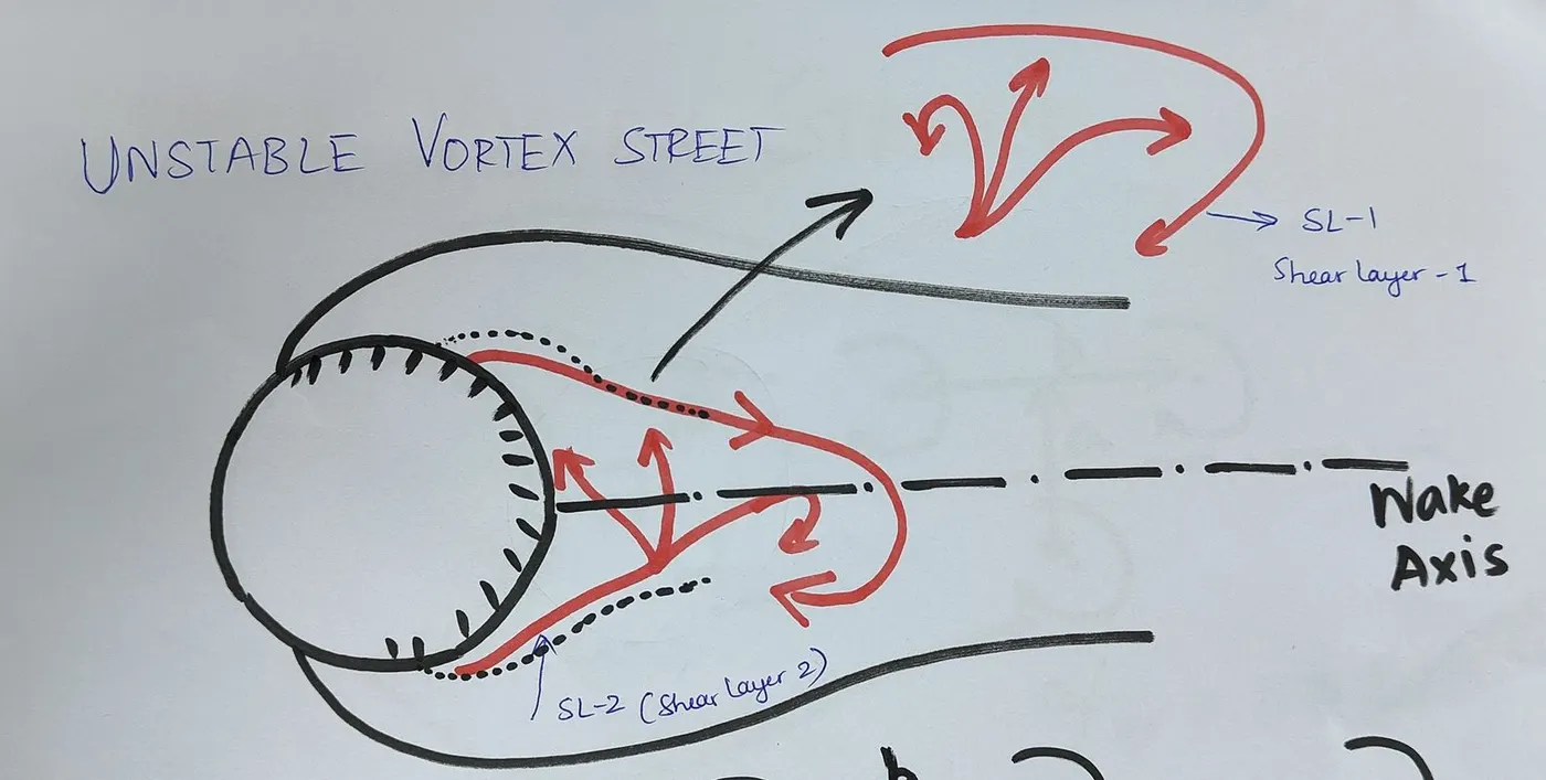
Considering top sheared layer to strecth more than the bottom sheared layer, this in turn creates a pressure suction in the bottom of the wake axis, hence the top sheared layer sucks the bottom vortices, and these layers are getting divided into various number of vortices conserving the pressure.
c) Vortex Visbilty Regimes
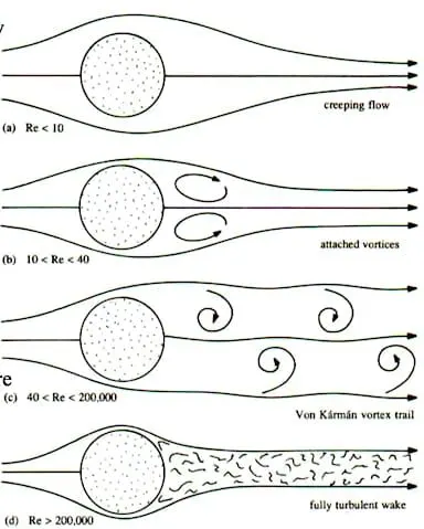
Vortices start shedding only for Reynolds number between 40 to 2,00,000, wherein after 2e5 Re , turbulen wake is generated.
2. Computational Domain
Click on Geometry to open SpaceClaim > Then draw a rectange of 60x20m, with a circle of 2m dimension at the 20m distance from the left face of the rectangle.
In order to pull the circle out from the Rectangle, Select > Pull > Click on the surface to pull away from the given surface
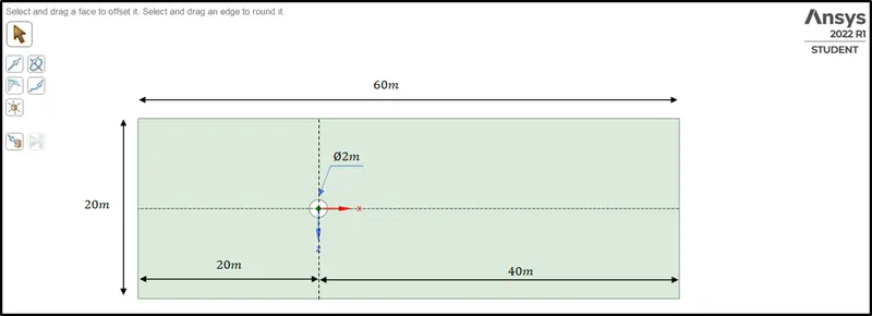
Now close geometry, get back to Workbench and update the geometry by right click and then update
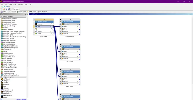
Now go to meshing, double click on meshing to open meshing
3. Meshing Methodologies
- First create Boundary Name for specifying Types of Boundary condition, so that ANSYS finds easy to put the boundary condition and select suitable solver
- Select Edge Selection > click on the edges and click 'N' as a shortcut to create Named Selection
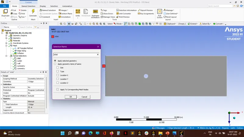
- After creating named selection Input, Output, wall (Edge of the circle) & Symmetry being the top and surface edges of the rectangle
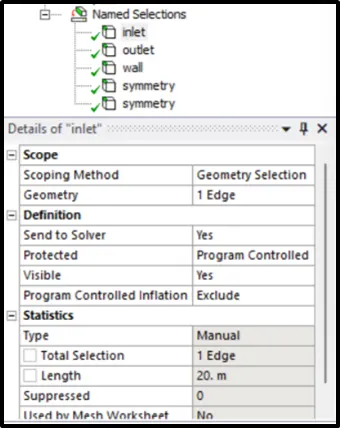
- Meshing elements of this geometry will be traingular elements, and in order to increase capture abilities at the cylindrical surface, we can increase it by using Inflation Layer
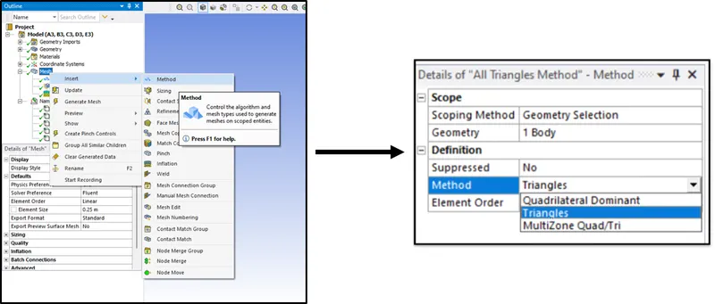
- Right click on Mesh > Insert > Methods > Select the surface of the geometry selection > Choose Method > Triangles
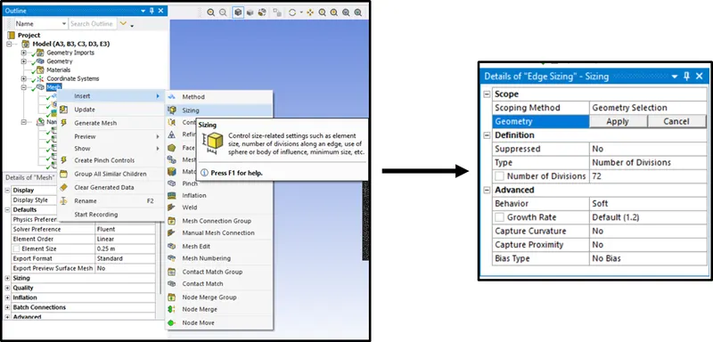
Sizing setup
- Right click on Mesh > Insert > Sizing > Select the surface of the geometry selection > Choose Geometry and Apply > Triangles
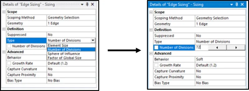
Then go to Type > Change type from Element size to Number of divisions to 72
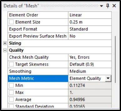
Global Mesh Element size setup
- Now keep the element size of the global mesh as 0.25m and select Quality as mesh metrics
Inflation Layer Setup
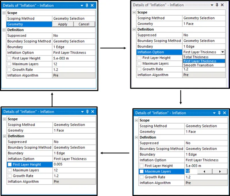
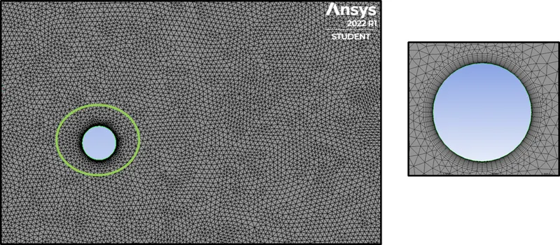
- Now go to Inflation > Select the Geometry > Apply > Go to Inflation Option > Select First Layer Thickness and enter the thickness value of the first layer as 5e-3m and no of layers as 12. Growth factor is maintained at 1.2. Keep it the same
Result after inflation layer setup:
4. Physics & Solver Setup
- Now close ANSYS Mesh > back to WB > Update Mesh in WB > Double click on the solver to open ANSYS Fluent
PART-I
- Simulate the flow with the steady and unsteady case and calculate the Strouhal Number for Re= 100.
For Re = 100
`R_e = frac(rho*v*d)(mu)`
where `mu = 0.02 (kg)/(ms)`
`rho = 1 (kg)/m^3`
`v = 1 m/s`
Once Fluent interface appears, you'll be able to se these many tools at the top of the Interface

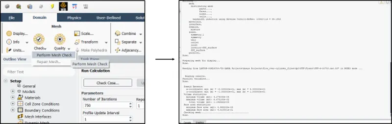
- Go to Domain > Check > Perform Mesh Check > Go to Console and check if the checking of mesh is complete
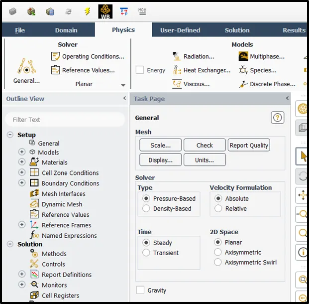
- Go to Physics > General Settings > Check whether it is Pressure Based solver indicating the fluid is incompressible in nature > Check Steady
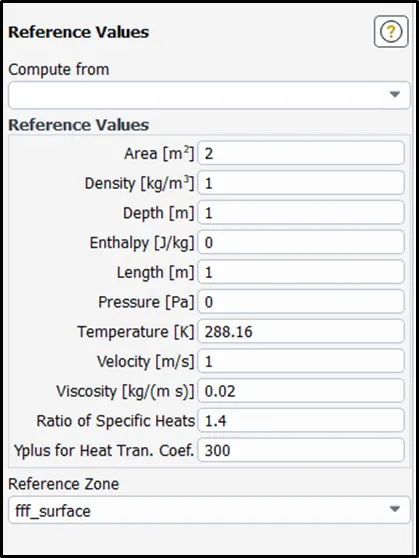
- Go to Physics > Reference Values > Edit the reference to get Reynolds to 100 by editing the Viscosity (Dynamic Viscosity) to 0.02 and edit the dimensional variables of area and length
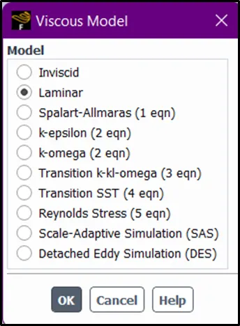
- Go to Physics > Viscous > Laminar
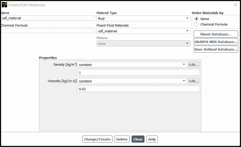
- Go to create/ edit materials > edit the database of material by clicking on Fluent Database > Create new material name > edit the properties of viscosity and density > delete the material of air installed by default in CELL ZONES
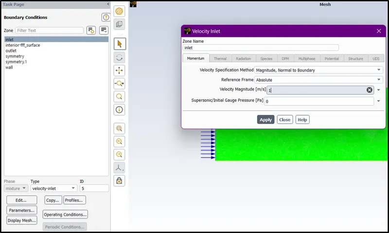
- Go to Boundary > Select Inlet > Edit the properties of Inlet Velocity to 1m/s > Keep the outlet to be pressure based for atmospheric guage pressure reading to 0 > Dont change other boundary conditions
- After setting up the solver and the physics > Make sure that the solution is done using SIMPLE (Semi implicit pressure linked equation) based scheme for physics involving fluid moving less than supersonic speeds
- For fluids moving at hypersonic and fast physics involvement one uses COUPLED Scheme
- Set pressure to be solved for Second order (Navier-Stokes Equation consiting of Second order tensors)
- Momentum equation to be resolved and discretized using UPWIND Scheme for second order
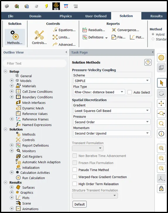
Creating Definitions for Plotting the quantities against No of iterations (Steady State)
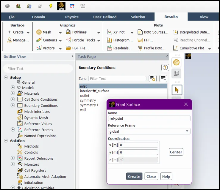
- Before going to Solutions and creating definitions, one must create a probe / monitor on the specific location of our domain to detect quantities of our definitions for this
- Go to Results > Create > Point-Surface > Give x = 8m, y = 0m and change name as per user
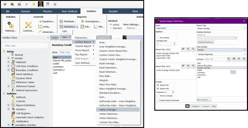
- After creating probe > Go to Solution > Definition > New > Surface Report > Vertex Average > Click on Velocity @ Probe > OK
- Now hit Hybrid Intilization > Initialize @ t=0
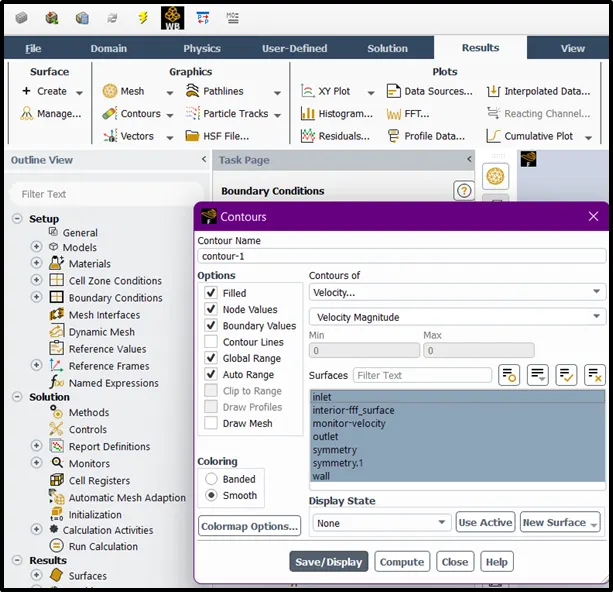
- After Initialization > Go to Results > Contours > New > Velocity and select all the boundary surfaces for Visualization of contours of specified quantities
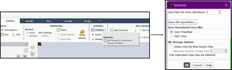
- Then go to Solutions > Auto-Save > Set frequency to capture solution of physics happening at every 5 iterations
- Enter number of Iterations as 750 and hit Calculate
NOTE :
1. For transient state solver change the solver from Steady to Transient in General physics solvers > Set time step size as t = 0.05s and total number of iterations for 500
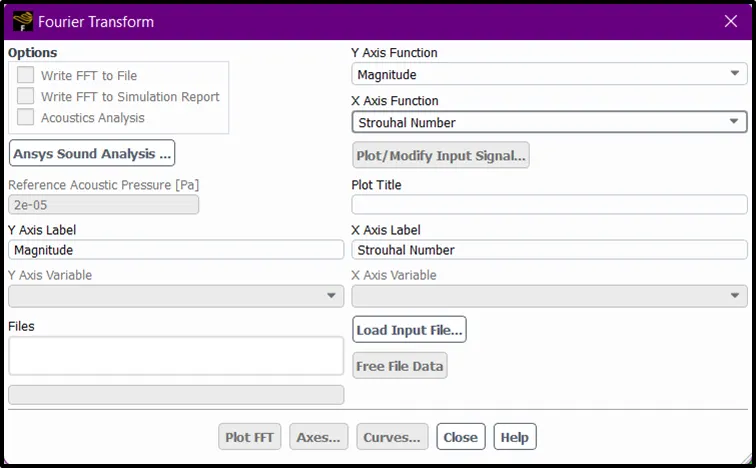
2. For Strouhal Number calculation
Go to Results > Plots > FFT > Change Y axis to Magnitude and X axis to Strouhal Number
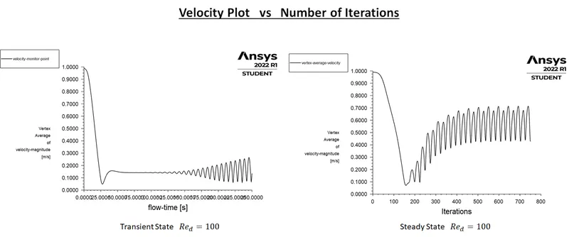
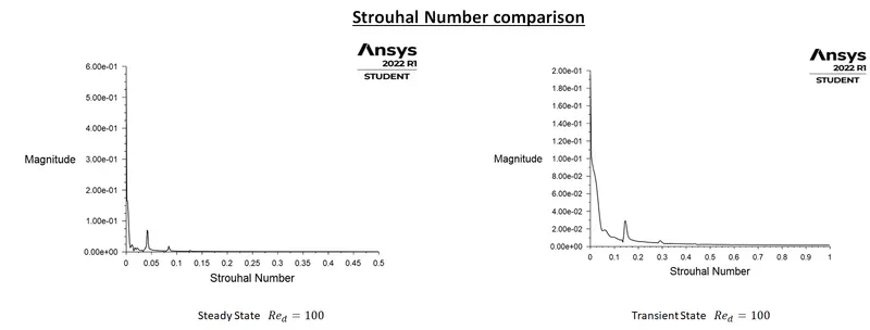
Results for Steady State & Transient solver
`R_e = 100`
To take a look at the obtained real time simulation, click on the links below
CASE I :
a) Steady State Solver - (Re = 100)
b) Tranisient State Solver - (Re = 100)
https://www.youtube.com/watch?v=Zfl_Frvgiis
CASE II :
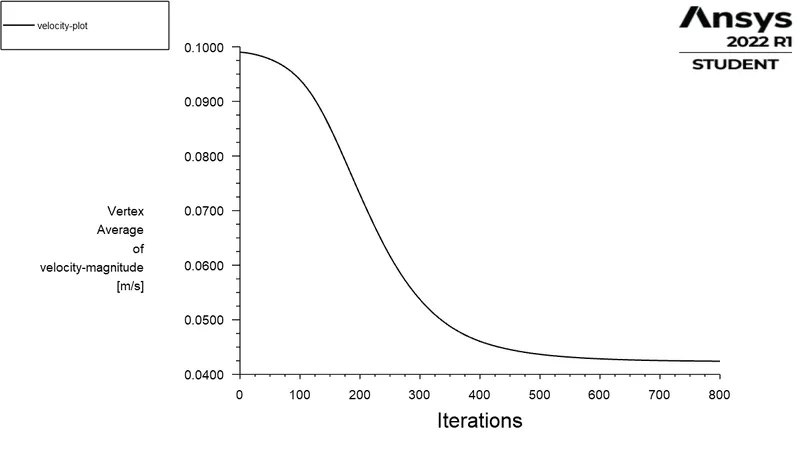
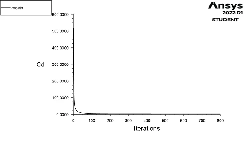
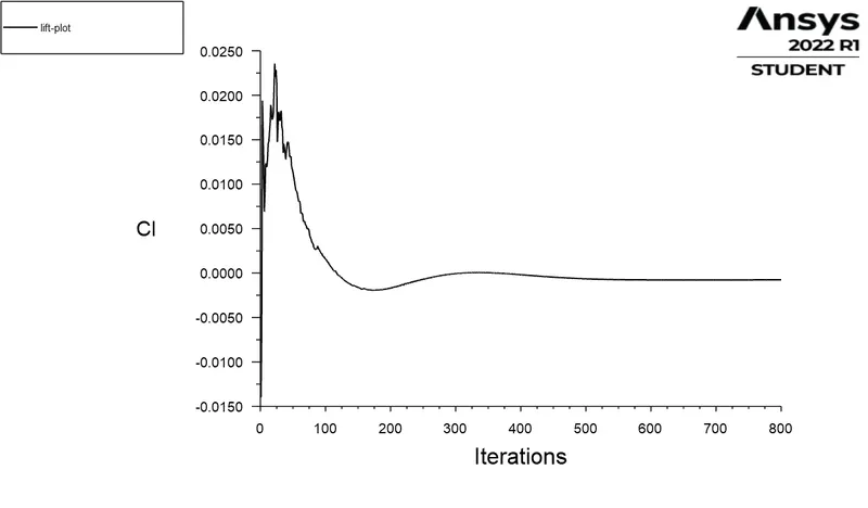
Results for Steady State solver
`R_e = 10`
i) Velocity Plot Distribution
ii) Drag-Coeffcient Plot Distribution
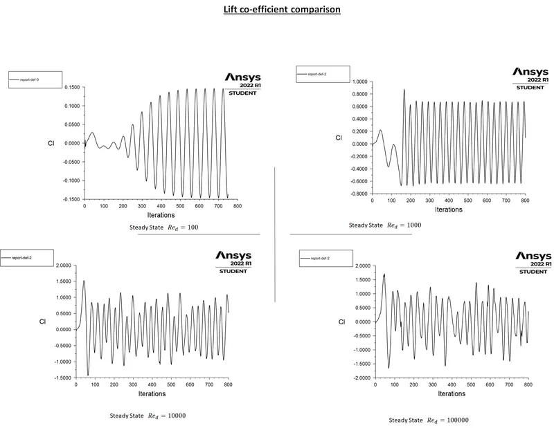
iii) Lift-Coeffcient Plot Distribution
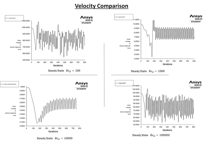
Results for Steady State solver
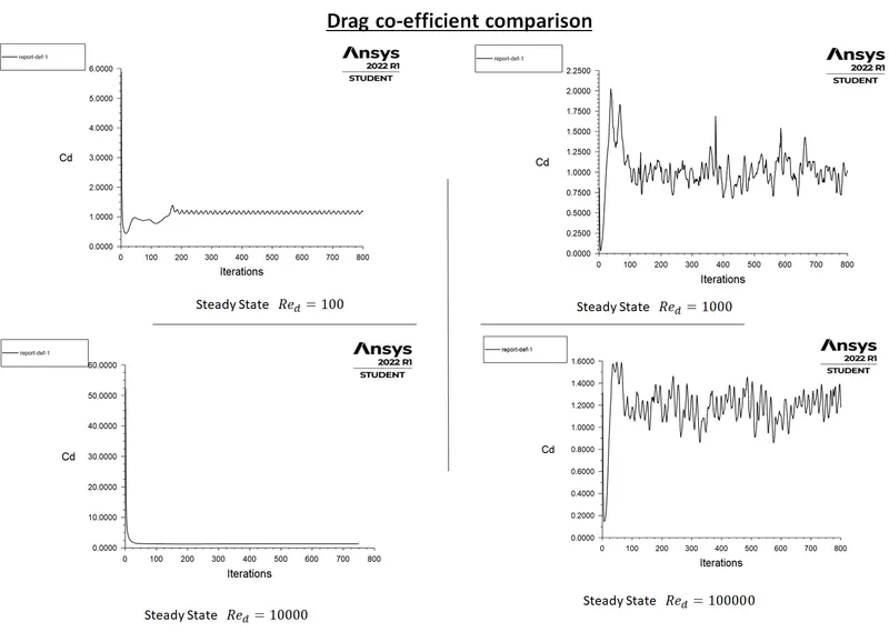
- `R_e = 100`
- `R_e = 1000`
- `R_e = 10000`
- `R_e = 100000`
i) Velocity Plot Distribution
ii) Drag-Coeffcient Plot Distribution
iii) Lift-Coeffcient Plot Distribution
CASE II :
To take a look at the obtained real time simulation, click on the links below
1. Steady State Solver for `R_e = 10`
2. Steady State Solver for `R_e = 100`
3. Steady State Solver for `R_e = 1000`
4. Steady State Solver for `R_e = 10000`
5. Steady State Solver for `R_e = 100000`
References :
1. Numerical Study of the Flow Over a Circular Cylinder in the Near Wake at Reynolds Number 3900 by
- HamiltonJet
2. Vortex shedding and its control by Prof. S.D.Sharma
3. Numerical simulation of laminar flow past a circular cylinder by B.N.RajaniaA.KandasamybSekharMajumdara