Week 3.5 - Deriving 4th order approximation of a 2nd order derivative using Taylor Table method

Objective : Deriving 4th order approximation of a 2nd order derivative using Taylor Table method

CASE I : Central Difference Scheme Approximation

Given :

The second order PDE for CDS is `frac{del^2f}{delx^2} = a*f_(i-2) + b.f'_(i-1) + c*f''_(i) + d.f'''_(i+1) + e.f''''_(i+2) rarr1`

Order of the derivative (Q) = 2

Order of Accuracy required (P) = 4

`:.` Number of Nodes (N) = P + (Q+1) For Symmetric CDS

Number of Nodes (N) = 7

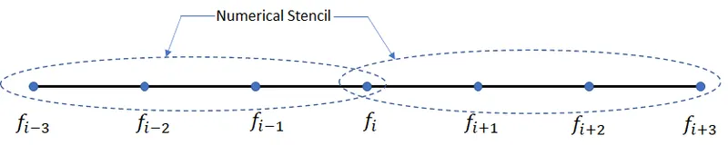
Expanding the PDE Terms of equation 1 using Taylor Series Expansion :

`a*f_(i-2) = a[f_(i) - (f'_(i)*frac{2Deltax}{1!}) + (f''_(i)*frac{(2Deltax)^2}{2!})-(f'''_(i)*frac{(2Deltax)^3}{3!}) + (f''''_(i)*frac{(2Deltax)^4}{4!}) - (f'''''_(i)*frac{(2Deltax)^5}{5!}) + (f''''''_(i)*frac{(2Deltax)^6}{6!})]`

`b*f_(i-1) = b[f_(i) - (f'_(i)*frac{Deltax}{1!}) + (f''_(i)*frac{(Deltax)^2}{2!})-(f'''_(i)*frac{(Deltax)^3}{3!}) + (f''''_(i)*frac{(Deltax)^4}{4!}) - (f'''''_(i)*frac{(Deltax)^5}{5!}) + (f''''''_(i)*frac{(Deltax)^6}{6!})`

`c*f_(i) = c*(f_(i))`

`d*f_(i+1) = d[f_(i) + (f'_(i)*frac{Deltax}{1!}) + (f''_(i)*frac{(Deltax)^2}{2!})+(f'''_(i)*frac{(Deltax)^3}{3!}) + (f''''_(i)*frac{(Deltax)^4}{4!}) + (f'''''_(i)*frac{(Deltax)^5}{5!}) + (f''''''_(i)*frac{(Deltax)^6}{6!})`

`e*f_(i+2) = e[f_(i) + (f'_(i)*frac{2Deltax}{1!}) + (f''_(i)*frac{(2Deltax)^2}{2!})+(f'''_(i)*frac{(2Deltax)^3}{3!}) + (f''''_(i)*frac{(2Deltax)^4}{4!}) + (f'''''_(i)*frac{(2Deltax)^5}{5!}) + (f''''''_(i)*frac{(2Deltax)^6}{6!})]`

Segregating co-efficients & evaluating using Taylor's Table :

	`f_i`	`f'_i*(frac{Deltax}{1!})`	`f''_i*(frac{Deltax^2}{2!})`	`f'''_i*(frac{Deltax^3}{3!})`	`f''''_i*(frac{Deltax^4}{4!})`	`f'''''_i*(frac{Deltax^5}{5!})`	`f''''''_i*(frac{Deltax^6}{6!})`
`a*f_(i-2)`	a	-2a	4a/2	-8a/6	16a/24	-32a/120	64a/720
`b*f_(i-1)`	b	-b	b/2	-b/6	b/24	-b/120	b/720
`c*f_(i)`	c	0	0	0	0	0	0
`d*f_(i+1)`	d	d	d/2	d/6	d/24	d/120	d/720
`e*f_(i+2)`	e	2e	4e/2	8e/6	16e/24	32e/120	64e/720
`sum`	0	0	1	0	0	To be determined	To be determined

Converting the above 5 equations to matrix form to evaluate 5 unknowns :

`[[1,1,1,1,1],[-2,-1,0,1,2],[2,1/2,0,1/2,2],[4/3,-1/6,0,1/6,4/3],[2/3,1/24,0,1/24,2/3]]*[[a],[b],[c],[d],[e]] = [[0],[0],[1],[0],[0]]`

`A = [[1,1,1,1,1],[-2,-1,0,1,2],[2,1/2,0,1/2,2],[4/3,-1/6,0,1/6,4/3],[2/3,1/24,0,1/24,2/3]]` , `X = [[a],[b],[c],[d],[e]]` & `B = [[0],[0],[1],[0],[0]]`

`:.` X = inv(A).B

Therefore performing Matrix Calculations in Matlab, we get the coefficients as follows :

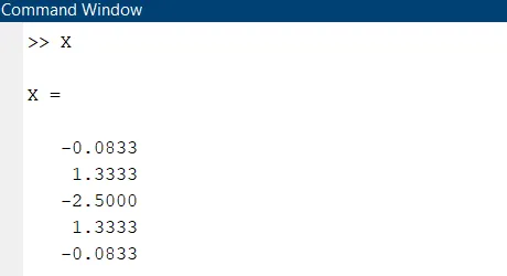
Substituting the values of matrix X in the below equation :

`frac{del^2f}{delx^2} = [(a+b+c+d+e)*f_i] + [(-2a-b+0+d+2e)*f_i'*Deltax] + [(frac{4a}{2} +b/2 +0+d/2+frac{4e}{2})*f_i''*Deltax^2] + [(-frac{8a}{6} -b/6 +0+d/6+frac{8e}{6})*f_i'''*Deltax^3 ]+[frac{16a}{24} + b/24 + 0 + d/24+ frac{16e}{24}*f_i''''*Deltax^4]+[(-frac{32a}{120} -b/120+0+d/120+frac{32e}{120})*f_i'''''*Deltax^5] +[(frac{64a}{720} +b/720 +0+d/720+frac{64e}{720})*f_i''''''*Deltax^6]`

`frac{del^2f}{delx^2} =[(frac{4a}{2} +b/2 +0+d/2+frac{4e}{2})*f_i''*Deltax^2]+[(frac{64a}{720} +b/720 +0+d/720+frac{64e}{720})*f_i''''''*Deltax^6]`

Dividing the RHS wrto `Deltax^2` :

`frac{del^2f}{delx^2} =[(frac{4a}{2} +b/2 +0+d/2+frac{4e}{2})*f_i'']+[(frac{64a}{720} +b/720 +0+d/720+frac{64e}{720})*f_i''''''*Deltax^4]`

Now we can clearly see that truncation error is in the order of `Deltax^4`.

Therefore we have proved that this is the CDS approximation for second order derivative with fourth order accuracy

_____________________________________________________________________________________________________________

CASE II : Skewed right-sided difference Scheme Approximation

Second order PDE is `frac{del^2f}{delx^2} = a*f_(i) + b.f'_(i+1) + c*f''_(i+2) + d.f'''_(i+3) + e.f''''_(i+4) + g.f''''''_(i+5) rarr1`

Order of the derivative (Q) = 2

Order of Accuracy required (P) = 4

`:.` Number of Nodes (N) = P + (Q) For skewed difference

Number of Nodes (N) = 6

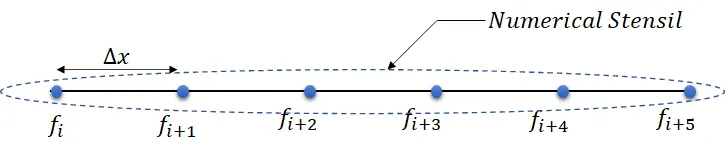
Expanding the PDE Terms of equation 1 using Taylor Series Expansion :

`a*f_(i) = a*(f_(i))`

`b*f_(i+1) = b[f_(i) + (f'_(i)*frac{Deltax}{1!}) + (f''_(i)*frac{(Deltax)^2}{2!})+(f'''_(i)*frac{(Deltax)^3}{3!}) + (f''''_(i)*frac{(Deltax)^4}{4!}) + (f'''''_(i)*frac{(Deltax)^5}{5!})`

`c*f_(i+2) = c[f_(i) + (f'_(i)*frac{2Deltax}{1!}) + (f''_(i)*frac{(2Deltax)^2}{2!})+(f'''_(i)*frac{(2Deltax)^3}{3!}) + (f''''_(i)*frac{(2Deltax)^4}{4!}) + (f'''''_(i)*frac{(2Deltax)^5}{5!})]`

`d*f_(i+3) = d[f_(i) + (f'_(i)*frac{3Deltax}{1!}) + (f''_(i)*frac{(3Deltax)^2}{2!})+(f'''_(i)*frac{(3Deltax)^3}{3!}) + (f''''_(i)*frac{(3Deltax)^4}{4!}) + (f'''''_(i)*frac{(3Deltax)^5}{5!})]`

`e*f_(i+4) = c[f_(i) + (f'_(i)*frac{4Deltax}{1!}) + (f''_(i)*frac{(4Deltax)^2}{2!})+(f'''_(i)*frac{(4Deltax)^3}{3!}) + (f''''_(i)*frac{(4Deltax)^4}{4!}) + (f'''''_(i)*frac{(4Deltax)^5}{5!})]`

`g*f_(i+5) = g[f_(i) + (f'_(i)*frac{5Deltax}{1!}) + (f''_(i)*frac{(5Deltax)^2}{2!})+(f'''_(i)*frac{(5Deltax)^3}{3!}) + (f''''_(i)*frac{(5Deltax)^4}{4!}) + (f'''''_(i)*frac{(5Deltax)^5}{5!})]`

Segregating co-efficients & evaluating using Taylor's Table :

	`f_i`	`f'_i*(frac{Deltax}{1!})`	`f''_i*(frac{Deltax^2}{2!})`	`f'''_i*(frac{Deltax^3}{3!})`	`f''''_i*(frac{Deltax^4}{4!})`	`f'''''_i*(frac{Deltax^5}{5!})`
`a*f_(i`	a	0	0	0	0	0
`b*f_(i+1)`	b	b	b/2	b/6	b/24	b/120
`c*f_(i+2)`	c	2c	4c/2	8c/6	16c/24	32c/120
`d*f_(i+3)`	d	3d	9d/2	27d/6	81d/24	243d/120
`e*f_(i+4)`	e	4e	16e/2	64e/6	256e/24	1024e/120
`g*f_(i+5)`	g	5g	25g/2	125g/6	625g/24	3125g/120
`sum`	0	0	1	0	0	0

Converting the above 6 equations to matrix form to evaluate 6 unknowns :

`[[1,0,0,0,0,0],[1,1,1/2,1/6,1/24,1/120],[1,2,4/2,8/6,16/24,32/120],[1,3,9/2,27/6,81/24,243/120],[1,4,16/2,64/6,256/24,1024/120],[1,5,25/2,125/6,625/24,3125/120]]*[[a],[b],[c],[d],[e],[g]] = [[0],[0],[1],[0],[0],[0]]`

`A = [[1,0,0,0,0,0],[1,1,1/2,1/6,1/24,1/120],[1,2,4/2,8/6,16/24,32/120],[1,3,9/2,27/6,81/24,243/120],[1,4,16/2,64/6,256/24,1024/120],[1,5,25/2,125/6,625/24,3125/120]] ` , `X = [[a],[b],[c],[d],[e],[g]]` & `B = [[0],[0],[1],[0],[0],[0]]`

`:.` X = inv(A').B`

Therefore performing Matrix Calculations in Matlab, we get the coefficients as follows :

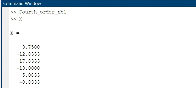
`frac{del^2f}{delx^2} = [(b/2 +frac{4c}{2}+frac{9d}{2}+frac{16e}{2}+frac{25g}{2})*f_i''*Deltax^2]+[(frac{b}{720}+frac{64c}{720}+ frac{729d}{720}+frac{4096e}{720}+frac{15625g}{720})*f_i''''''*Deltax^6]`

Dividing the RHS wrto `Deltax^2` :

`frac{del^2f}{delx^2} = [(b/2 +frac{4c}{2}+frac{9d}{2}+frac{16e}{2}+frac{25g}{2})*f_i'']+[(frac{b}{720}+frac{64c}{720}+ frac{729d}{720}+frac{4096e}{720}+frac{15625g}{720})*f_i''''''*Deltax^4]`;

Now we can clearly see that truncation error is in the order of `Deltax^4`.

Therefore we have proved that this is the Skewed right-sided difference Scheme approximation for second order derivative with fourth order accuracy.

________________________________________________________________________________________________________________________________

CASE III : Skewed Left-sided difference Scheme Approximation

Second order PDE is `frac{del^2f}{delx^2} = a*f_(i-5) + b.f'_(i-4) + c*f''_(i-3) + d.f'''_(i-2) + e.f''''_(i-1) + g.f'''''_(i) rarr1`

Order of the derivative (Q) = 2

Order of Accuracy required (P) = 4

`:.` Number of Nodes (N) = P + (Q) For skewed difference

Number of Nodes (N) = 6

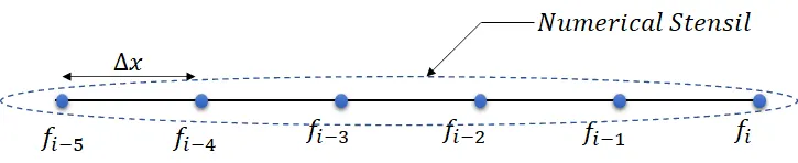
Expanding the PDE Terms of equation 1 using Taylor Series Expansion :

`g*f_(i) = g*(f_(i))`

`e*f_(i-1) = e[f_(i) - (f'_(i)*frac{Deltax}{1!}) + (f''_(i)*frac{(Deltax)^2}{2!})-(f'''_(i)*frac{(Deltax)^3}{3!}) + (f''''_(i)*frac{(Deltax)^4}{4!}) - (f'''''_(i)*frac{(Deltax)^5}{5!})`

`d*f_(i-2) = d[f_(i) - (f'_(i)*frac{2Deltax}{1!}) + (f''_(i)*frac{(2Deltax)^2}{2!})-(f'''_(i)*frac{(2Deltax)^3}{3!}) + (f''''_(i)*frac{(2Deltax)^4}{4!}) - (f'''''_(i)*frac{(2Deltax)^5}{5!})]`

`c*f_(i-3) = c[f_(i) - (f'_(i)*frac{3Deltax}{1!}) + (f''_(i)*frac{(3Deltax)^2}{2!})-(f'''_(i)*frac{(3Deltax)^3}{3!}) + (f''''_(i)*frac{(3Deltax)^4}{4!}) - (f'''''_(i)*frac{(3Deltax)^5}{5!})]`

`b*f_(i-4) = b[f_(i) - (f'_(i)*frac{4Deltax}{1!}) + (f''_(i)*frac{(4Deltax)^2}{2!})-(f'''_(i)*frac{(4Deltax)^3}{3!}) + (f''''_(i)*frac{(4Deltax)^4}{4!}) - (f'''''_(i)*frac{(4Deltax)^5}{5!})]`

`a*f_(i-5) = a[f_(i) - (f'_(i)*frac{5Deltax}{1!}) + (f''_(i)*frac{(5Deltax)^2}{2!})-(f'''_(i)*frac{(5Deltax)^3}{3!}) + (f''''_(i)*frac{(5Deltax)^4}{4!}) - (f'''''_(i)*frac{(5Deltax)^5}{5!})]`

Segregating co-efficients & evaluating using Taylor's Table :

	`f_i`	`f'_i*(frac{Deltax}{1!})`	`f''_i*(frac{Deltax^2}{2!})`	`f'''_i*(frac{Deltax^3}{3!})`	`f''''_i*(frac{Deltax^4}{4!})`	`f'''''_i*(frac{Deltax^5}{5!})`
`a*f_(i-5)`	a	-5a	25a/2	-125a/6	625a/24	-3125a/120
`b*f_(i-4)`	b	-4b	16b/2	-64b/6	256b/24	-1024b/120
`c*f_(i-3)`	c	-3c	9c/2	-27c/6	81c/24	-243c/120
`d*f_(i-2)`	d	-2d	4d/2	-8d/6	16d/24	-32d/120
`e*f_(i-1)`	e	-e	e/2	-e/6	e/24	-e/1
`g*f_(i)`	g	0	0	0	0	0
`sum`	0	0	1	0	0	0

Converting the above 6 equations to matrix form to evaluate 6 unknowns :

`[[1,1,1,1,1,1],[-5,-4,-3,-2-,1,0],[25/2,16/2,9/2,4/2,1/2,0],[-125/6,-64/6,-27/6,8/6,-1/6,0],[625/24,256/24,81/24,16/24,1/24,0],[-3125/120,-1024/120,-243/120,-32/120,-1/120,0]]*[[a],[b],[c],[d],[e],[g]] = [[0],[0],[1],[0],[0],[0]]`

`A = [[1,1,1,1,1,1],[-5,-4,-3,-2-,1,0],[25/2,16/2,9/2,4/2,1/2,0],[-125/6,-64/6,-27/6,8/6,-1/6,0],[625/24,256/24,81/24,16/24,1/24,0],[-3125/120,-1024/120,-243/120,-32/120,-1/120,0]] ` , `X = [[a],[b],[c],[d],[e],[g]]` & `B = [[0],[0],[1],[0],[0],[0]]`

`:.` X = inv(A).B`

Therefore performing Matrix Calculations in Matlab, we get the coefficients as follows :

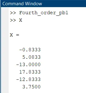
`frac{del^2f}{delx^2} = [(frac{25a}{2} +frac{16b}{2}+frac{9c}{2}+frac{4d}{2}+frac{e}{2}+0)*f_i''*Deltax^2]+(k)*f_i''''''*Deltax^6`

Dividing the RHS wrto `Deltax^2` :

`frac{del^2f}{delx^2} = [(frac{25a}{2} +frac{16b}{2}+frac{9c}{2}+frac{4d}{2}+frac{e}{2}+0)*f_i]+(k)*f_i''''''*Deltax^4`

Now we can clearly see that truncation error is in the order of `Deltax^4`.

Therefore we have proved that this is the Skewed left-sided difference Scheme approximation for second order derivative with fourth order accuracy.

_________________________________________________________________________________________________________________________

OBJECTIVE :

To evaluate the second-order derivative of the analytical function exp(x)*cos(x) and compare it with the 3 numerical approximations

`f(x) = e^x*cos(x)`

`ddotf(x) = -2*e^x*sin(x) rarr Exact Derivative`

Matlab function to evaluate 2nd order derivative (Central differencing) :

function error_cds = fourth_order_cds(x,dx)

exact_derivative = -2*exp(x)*sin(x);

cds = ((-0.0833)*((exp(x-(2*dx)))*(cos(x-(2*dx)))))+((1.3333)*((exp(x-dx))*((cos(x-dx))))-((2.5000)*((exp(x))*(cos(x))))+((1.3333)*((exp(x+dx))*(cos(x+dx))))-((0.0833)*((exp(x+(2*dx)))*(cos(x+(2*dx))))))/(dx^2); 

error_cds = abs(cds - exact_derivative);
end

Matlab function to evaluate 2nd order derivative (Right side skewed differencing) :

function error_srds = fourth_order_srds(x,dx)

exact_derivative = -2*exp(x)*sin(x);

srds = (((3.75)*((exp(x))*(cos(x))))-((12.833)*((exp(x+dx))*(cos(x+dx))))+((17.833)*((exp(x+2*dx)))*(cos(x+(2*dx)))))-((13)*((exp(x+(3*dx)))*(cos(x+(3*dx))))) + ((5.0833)*((exp(x+(4*dx)))*(cos(x+(4*dx)))))-((0.833)*((exp(x+(5*dx)))*(cos(x+(5*dx)))))/(dx^2);

error_srds = abs(srds - exact_derivative);
end

Matlab function to evaluate 2nd order derivative (Left side skewed differencing) :

function error_srds = fourth_order_slds(x,dx)

exact_derivative = -2*exp(x)*sin(x);

slds = ((-0.0833)*((exp(x-(5*dx)))*(cos(x-(5*dx)))))+((5.0833)*((exp(x-(4*dx)))*((cos(x-(4*dx)))))-((13.000)*((exp(x-(3*dx)))*(cos(x-(3*dx)))))+((17.8333)*((exp(x-(2*dx)))*(cos(x-(2*dx)))))-((12.833)*((exp(x-dx))*(cos(x-dx))))+((3.750)*((exp(x))*(cos(x)))))/(dx^2);
error_srds = abs(slds - exact_derivative);
end

Comparing three schemes using range of grid sizes and computing in Matlab :

close all
clear all
clc

x =pi/3;
dx = linspace(pi/4,pi/4000,20);

for i = 1:length(dx)
    central_diff(i) = fourth_order_cds(x,dx(i));
    right_skew(i) = fourth_order_srds(x,dx(i));
    left_skew(i) = fourth_order_slds(x,dx(i));
end

figure(1)
loglog(dx,central_diff,'color','r');
hold on
grid on
loglog(dx,right_skew,'color','k');
loglog(dx,left_skew,'color','g');
xlabel('Grid Size');
ylabel('Error');
legend('Central Difference Scheme','Right Skew Scheme','Left Skew Scheme','location','North west')

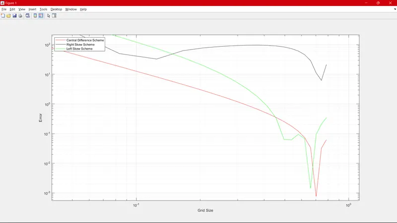
Result :

Conclusion :

* Central differencing approximation scheme is showing less error and tends to reduce much more quickly than other two schemes

* Due to usage of points on both the axis of stensil, CDS is able to provide a higher accurate value for the numerical derivative

Why Skewed Schemed is useful ?

* CDS requires nodes on both sides of stensil while skewed schemes can manage with less data compromising the accuracy of the numerical derivative

What can a skewed scheme do that a CD scheme cannot?

* CDS cannot be used where conditions of using nodes only in one side of the stensil is present such as boundary nodes where there are no left & right nodes present. At this situation skewed schemes tend to be much useful