Week 4 - CHT Analysis on Exhaust port

CHT Analysis on Exhaust port

Why and where CHT is used ?

The Conjugate Heat Transfer (CHT) analysis type allows for the simulation of heat transfer between solid and fluid domains by exchanging thermal energy at the interfaces between them. Typical applications of this analysis type exist as, but are not limited to, the simulation of heat exchangers, cooling of electronic equipment, and general-purpose cooling and heating systems.

STEP I : Geometry Preparation & Volume Extraction

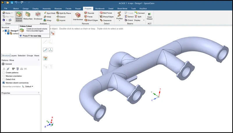
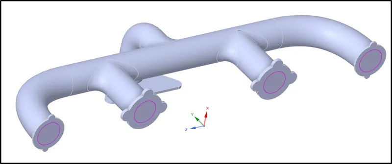
• Go to Prepare > Edge Selection > Click on the Inlet Edges & Outlet Edges

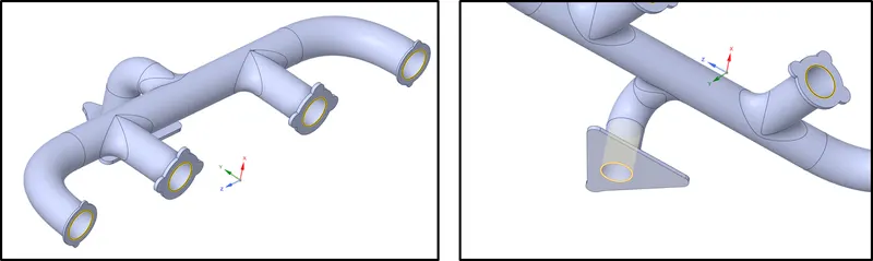
• Rename the Volume as 'Wet Volume'
  
• Rename th remaining Volume as 'Solid Volume'

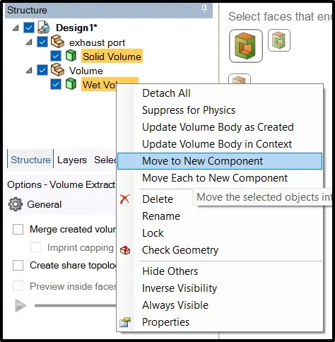
• Click on these 2 Named Volumes > Righrt Click to create a seperate folder named 'Total Geometry'

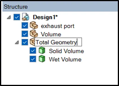
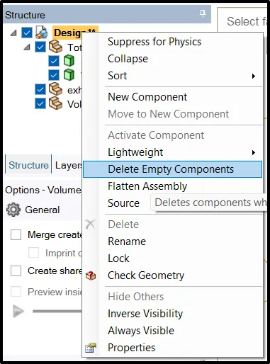
• Right Click on FF Geometry to delete empty components for no other confusion in PID generation

Conformal Meshing Preparation :

Enabling Sharing Topology from one PID to other for shring for physical properties like temperature, heat transfer flux etc

• Workbench > Drag & Select the whole geometry > Wait for Overlap & Shadow preparation

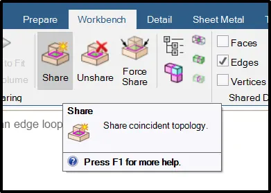
• If Pink circles appears on the edges of Inlet & Outlet Geometry then 'Share Topology' is enabled

STEP II : Meshing

Near Wall bounded flows :

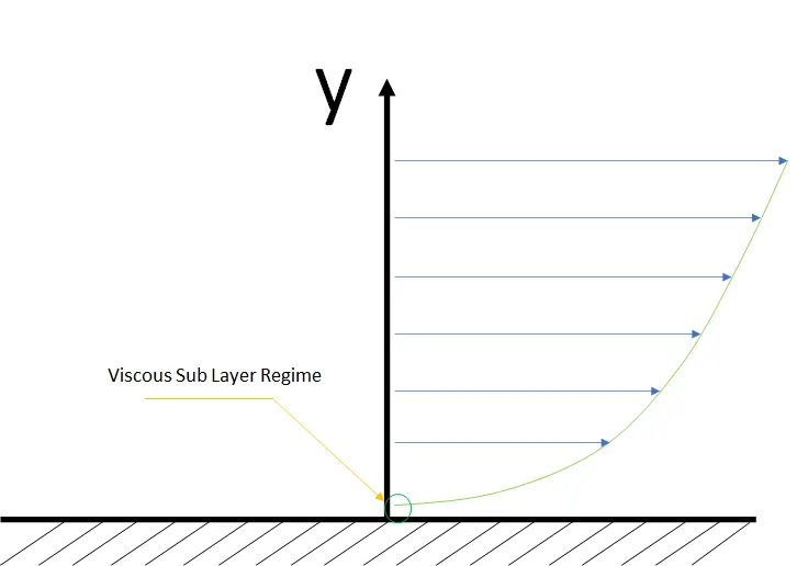
Wall Shear Stress

`tau_(wall)` = `mu*frac{du}{dy}`

`tau_(wall)` = `mu*frac{overlineu}{y}`

Expressing `tau_(wall)`in terms of Velocity Dimensions

`rho*u_(tau)^2 = mu*frac{overlineu}{y}`

`rho*u_(tau)*u_(tau) = mu*frac{overlineu}{y}`

`frac{overlineu}{u_(tau)} = frac{y*rho*u_(tau)}{mu}`

`[frac{overlineu}{u_(tau)}] = [frac{y}{mu/(rho*u_(tau))}]`

`[frac{overlineu}{u_(tau)}] = u^(+)`

`[frac{y}{mu/(rho*u_(tau))}] = y^(+)`

Very Near to the wall :

`u^+ = y^+`

At inner regime (Viscous-sub layer) :

`u^+ =f( y^+)`

At outer regime (Turbulent layer) :

`[frac{overlineu-u_infty}{u_tau}] = f(eta)`

where `eta = y/delta` - Length Scale of Viscosity

This deviation of `overlineu` from the free stream velocity is due to turbulent stresses from the equation `overline(rho*u_i*u_j)` from Reynolds averaging after decompositon. This is known as the Velocity Defect Law

Considering contnuity of du & dy at both inner & outer layer:

`frac{doverlineu}{dy}| = frac{doverlineu}{dy}|_(outer)`

Switching from `overlineu` to `u^+` since its function of one another:

`frac{du^+}{dy}*frac{dy^+}{dy} =` `frac{doverlineu}{dy}`

`frac{du^+}{dy}*(frac{rho*u_(tau)}{mu}) =frac{du^+}{d eta}*frac{d eta}{dy}`

where

`eta = y/delta` and `(d eta)/(dy) = 1/delta`

`frac{du^+}{dy}*(frac{rho*u_(tau)}{mu}) =frac{du^+}{d eta}*frac{1}{delta}`

Multiply y on both sides of the equation :

`frac{du^+}{dy}*(y^+) =frac{du^+}{d eta}*(eta)`

where both the terms are treated to be constants

`frac{du^+}{dy}*(y^+)` - Term I

`frac{du^+}{d eta}*(eta)` - Term II

Rearranging the terms for Integration wrto `y^+` :

`du^+` = `1/y^+ * dy^+`

First Term after Integration :

`u^+ = (1/k) * lny^+ + B`

where the value of k is empirically calculated to be k`approx0.5`

and value of B is empirically calculated to be B`approx5`

This is called the Law of the Wall

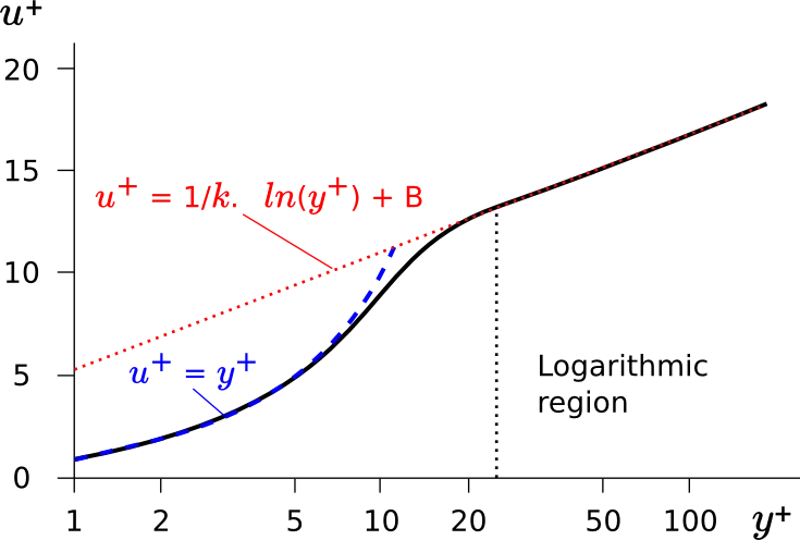
0 < `y^+` < 5 - Vicous Sub Layer Regime

5 < `y^+` < 30 - Buffer Layer Regime

`y^ + `> 30 - Turbulent Layer Regime

Calculation of `y^ + `

Given Data from Boundary Conditions

u = 5 m/s

L = 0.166m

`rho` = 1.225 kg/m3

`mu` = 1.7984 kg/ms

Calculation of Reynold's Number :

`Re_L = (rho*v*L)/(mu)`

`Re_L` = 56854.95

Calculation of Skin Friction co-efficient :

`C_f = 0.079*(Re)^-0.25`

`C_f ` = 0.005116

Calculation of Wall Shear Stress :

`tau_(wall) = (C_f*rho*v^2)/(2)`

`tau_(wall)` = 0.0783 N

Calculation of Frictional Velocity :

`U_f = sqrt((tau_(wall))/(rho))`

`U_f ` = 0.2528 m/s

Calculation of First Cell height :

`y^+ = [(rho*U_f*y)/mu]`

`y = [(mu*y^+)/(rho*U_f)]`

CASE I : For `k-omega` SST Model

Input `y^+` = 5

`y = [(mu*y^+)/(rho*U_f)]`

`y = [((1.7894e-5)*(5))/((1.225)*(0.2528))]`

y = 0.3195 mm

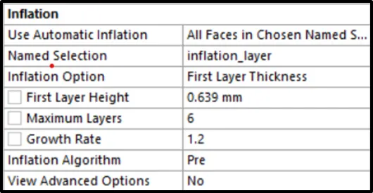
First Cell Height for `k-omega` SST Model

yx2 = 0.639 mm

CASE II : For `k-epsilon`Model

Input `y^+` = 10

`y = [(mu*y^+)/(rho*U_f)]`

`y = [((1.7894e-5)*(10))/((1.225)*(0.2528))]`

y = 0.639 mm

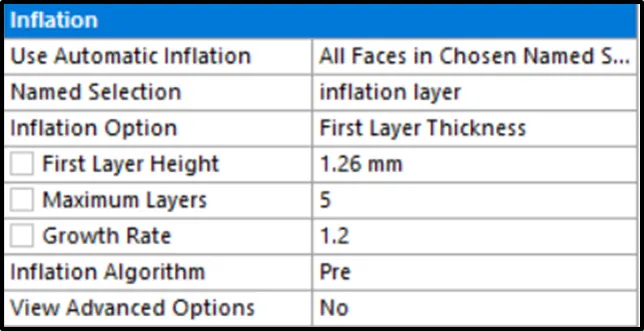
First Cell Height for `k-epsilon`

yx2 = 1.26 mm

Meshing Methodology :

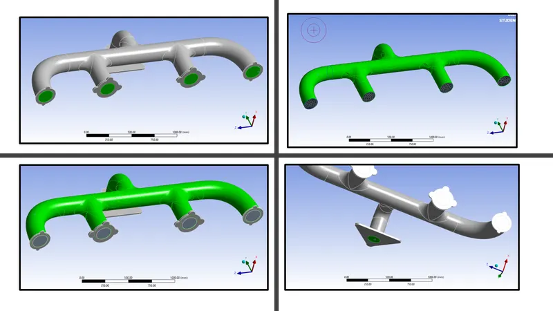
> Open the file

> Right select for 'Create a named Selection' or Click N

> Select Inlets faces ->"Inlet"

> Select Outlet face -> "Outlet"

> Double the face of the body -> "Outer Wall Convection"

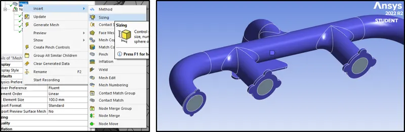
> Intialize the mesh with 100mm as the element size

> Then right click Mesh -> Body Sizing -> Select the "Outer Wall Convection" PID by drag select using Body Selection

> Enter Body size options for element size as 50mm

Meshing Results :

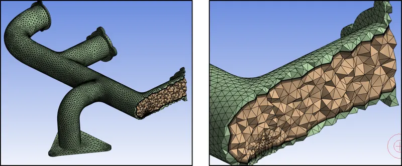
For `k-epsilon` Model :

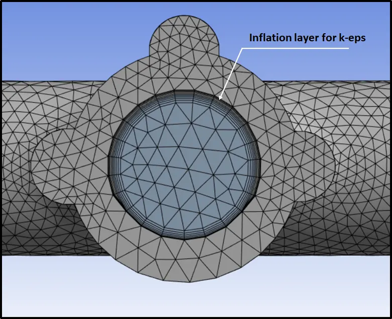
Total no of elements = 236735

For `k-omega` Model :

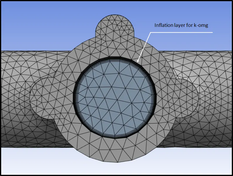
Total no of elements = 260118

Solving Methodology :

> Open Fluent after updating Meshing

> Check Mesh once interface is loaded

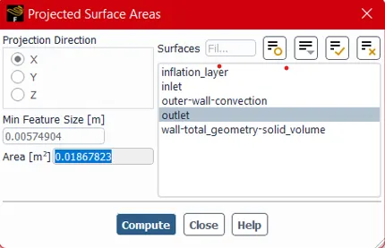
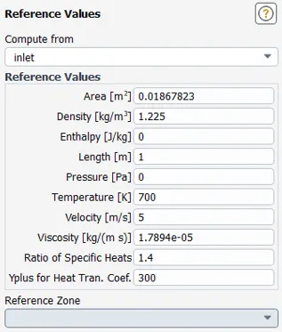
> Go to Reference Values, calculate projected refrence areas

> Input right boundary value (Velocity @ Inlet ; Temp @ inlet)

> Turn on the Energy Equation, since we are dealing with temperature in our system (Convection-Diffusion Modelling)

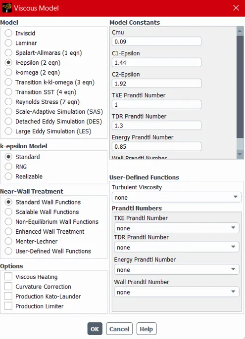
> Click on Viscous Model -> go to k-eps turbuence modelling -> Standard/Realizable model (for capturing swirl in action use RNG Model)

> Go to Material Properties check for fluid material as AIR and solid material as AL

> Boundary Conditions

• Inlet = 5m/s ; Inlet Temp = 700K
• Outlet = Pressure based ; ATM PRESSURE = 1 BAR ; GAUGE PRESSURE = 0
• Outer wall = Convection -> HTC = 20`W/(m^2K)`

> Solution Methods

• SIMPLE SCHEME

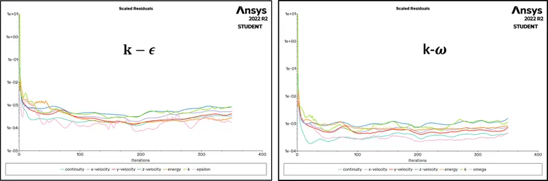
> Reduce all convergence criterias for residuals to 0 for better accurate results for longer iterations

> Generate report definitions for

• Static Temperature @ Outer wall convection
• Heat Transfer co-efficient @ Inflation layer shadow

> Intiate the solution

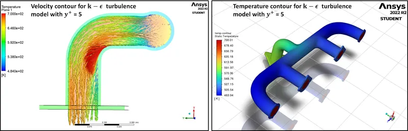
> Generate a contour for Temperature for the geometry

> Generate a contour for a XY Plane at the Exhaust Pipe for velocity contour

> Calculations for 350 Iterations

Results (Plots) :

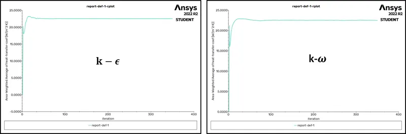
• Average Temperature at Outer wall

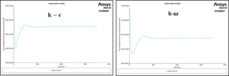
• Average Heat Transfer Co-efficient

• Residuals

Results (Contours) :

For `k-epsilon` Model :

• HTC Contour for `k-epsilon` Model :

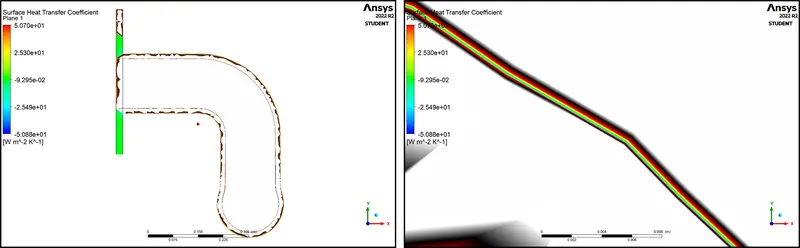
• HTC Contour for `k-omega` Model
  

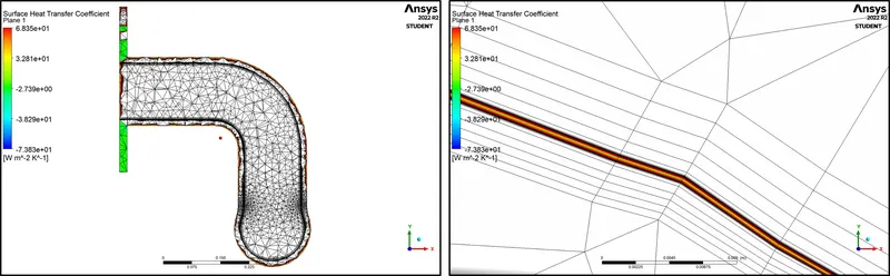
Verification of HTC predections from the simulation can be done in following ways:

1. By numerical way. It can be done by calculating Nusselts number and heat transfer coefficient and comparing with the results obtained from the simulation.

where,

h = convective heat transfer coefficient of the flow

L = characteristic length

k = thermal conductivity of the fluid.

For free convection, the average Nusselt number is expressed as a function of the Rayleigh number and the Prandtl number, written as:

Otherwise, for forced convection, the Nusselt number is generally a function of the Reynolds nuumber and the Prandtl number, written as:

2. By experimental analysis, the experiment should be conducted for the simulation done and by compairing both output results, validation of performed analysis can be done.

Factors on which prediction accuracy depends:

1. Meshing the geometry with finer mesh as much as possible and Inflation layer must be given wherever required.

2. Topology for the different volumes must be shared in the geometry for node to node coneection in meshing which will be responsible for more accurate results.

3. Selection of solution models, methodology etc also affect the precition accuracy.