Week 9 - FVM Literature Review
Finite Volume Method (A hybrid of FDM & FEM)
Motivation from limitations of Finite difference method (FDM)
What kind of behaviour do we desire from a discretizion method for solving good CFD problems ?
1. Conservativeness
2. Boundedness
3. Transportiveness
Conservativeness
A governing differential equation for a property `phi` is conservative in nature over its differential & integral forms.
Let us say that the property `phi` must conserve momentum along all axes over its domain. In order find numerical solutions for momentum equation for property `phi`, one follows the discretization methods like FDM, FEM & FVM as follows to convert the differential form of equations to algebraic form for finding the solution.
The produced discretized form of the governing differential equation must also be conservative in nature over its domain, i,e the sum of all discretized forms of the gde must obey the conservation of momentum.
Whereas the FDM method by its nature doesnt enforce any inbuilt conservativeness in its method. Since FDM involves a taylor's table technique to find the values of property along direction & time.
Accuracy
`f(x+h) = f(x) + f'(x)*h + f''(x)*h^2/(2!) + .......+ f^(n-1)(x)*h^(n-1)/((n-1)!)`
By intuition, the higher order terms of Taylor series are usually truncated assuming that the values of 'h' decreases as it increases for higher order terms, which is a major disadvantage for function whose variation terms vary by `e^x`equation.
Since derivative of the term `e^x`itself is the function, one cannot ignore the terms by truncating it. This surely deviates the solution from the exact solution.
The requirement for positive coefficients in the central differencing scheme implies that the scheme will be stable and accurate only if Pe = F/D < 2. It is important to note that the cell Peclet number is a combination of fluid properties (ρ and Γ), a flow property (u) and a property of the computational grid (δx). So for given values of ρ and Γ it is only possible to satisfy condition if the velocity is small, hencein diffusion-dominated low Reynolds number flows, or if the grid spacing is
small. Owing to this limitation central differencing is not a suitable discretisation practice for general-purpose flow calculations. T
Boundedness
Let us consider a rod which is in contact with ice at left end and at steam at the right end. If we are interested to plot a temperature distribution of the rod along the length (l), the temperature interface values of the rod must not go beyond the boundary values of the domain. This has to ensured by the physical nature of the governing differential equation & so does the discretized form of the g.d.e. But ultimately, FDM method doesnt employ any such boundedness by its method.
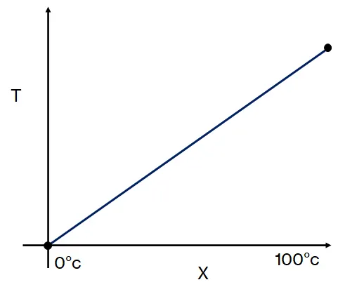
Finite Volume method :
STEP I : Divide the domain into number of finite sized sub-domain called Control Volume. Each sub-domain is represented by a finite number of grid points
STEP II : Integrate g.d.e over each sub-domain
STEP III : Consider profile assumption (Interpolation function) for the dependent variable for evaluating above integrals to express result interms of algebraic quantities at grid points.
Illustrative example for FVM discretization for Steady State Convection-Diffusion equation
General transport equation for property `phi` is given by
`frac{del(rho*phi)}{delt} + nabla*(rho*phi*U) = nabla(Gamma*nablaphi) + S`
The governing equation of steady diffusion can easily be derived from the general transport equation
`int_(cv)nabla(Gamma*nablaphi) + int_(cv)S_phi = 0`
Now integrating the g.d.e over the control volume
`int_(cv)nabla(Gamma*nablaphi)*dv + int_(cv)S_phi*dv = 0`
Using divergence theorem, converting the volume integrals to surface integrals to calculate fluxes
`int_(cs)eta*(Gamma*A*nablaphi)*ds + int_(cv)S_phi = 0`
The control volume method itself is conservative in nature, since the g.d.e are conservative, the equation itself is integrated over the whole domain making sure that the conservation is applied throughout the control volume
Working with the one-dimensional steady state diffusion equation, theapproximation techniques that are needed to obtain the so-called discretisedequations are introduced.
Standard representation of Control Volume :
Control volume and its properties are present at the centroid of the volume irrespective of its shape. Since it is an easy location to be found.
These centroids are called the grid points / nodal points of the control volume which are surrounded by its control surfaces respectively.
Control surface on the left is termed as west face denoted as 'w' & right face as 'r' respectively. The grid point in focus of calculation is determined by 'P' & the neighbouring grid point to the left is denoted as 'W' & to the right as 'R' respectively.
Boundaries of the domain are denoted as A & B respectively
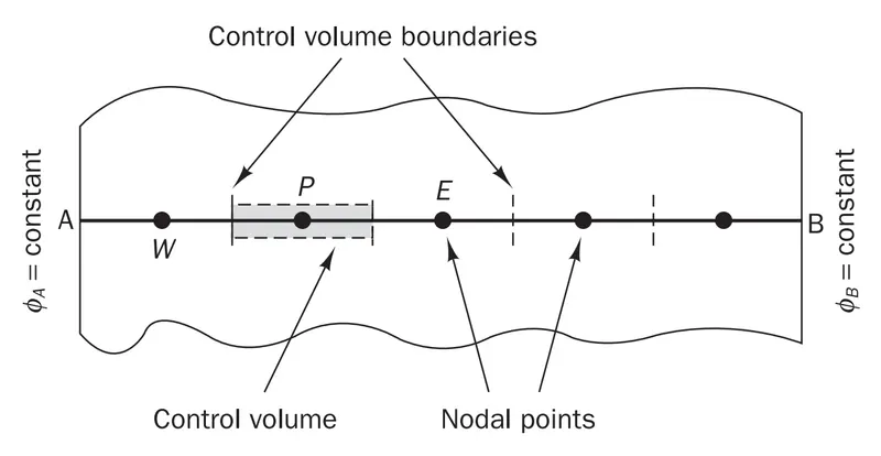
Distance between centroid grid point of the control volume and its control surface are given in the figure below
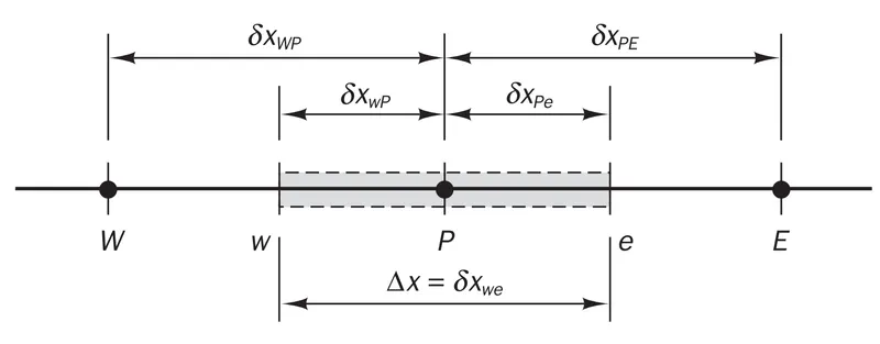
Illustrative Example using FVM for numerical analysis of 1-D Steady state heat conduction equation
1-D Steady state conduction with constant heat source
`frac{d}{dx}(k*frac{dt}{dx}) +(S) = 0`
STEP I : Divide the domain into number of sub domains

STEP II : Integarting the g.d.e over each control volume
`int_w^efrac{d}{dx}(k*frac{dt}{dx})*dx +int_w^e(S*dx) = 0`
Since S is a constant, can be taken out of the iintegral
`[k*frac{dt}{dx}]_e - [k*frac{dt}{dx}]_w + S*int_w^e(dx) = 0`
`[k*frac{dt}{dx}]_e - [k*frac{dt}{dx}]_w + S*(x_e - x_w) = 0`
`[k*frac{dt}{dx}]_e - [k*frac{dt}{dx}]_w + S*(Deltax) = 0`
`[k*frac{dt}{dx}]_e - [k*frac{dt}{dx}]_w + S*(Deltax) = 0`
`:.` By central differencing scheme, converting differential equation to algebraic
`k_e*[frac{T_E - T_P}{deltax_(PE)}] - k_w*[frac{T_P - T_W}{deltax_(WP)}]+ S*(Deltax) = 0`
`[frac{k_e}{deltax_(PE)} + frac{k_w}{deltax_(WP)}]*T_P = [frac{k_e}{deltax_(PE)}]*T_E + [frac{k_w}{deltax_(WP)}]*T_W + S*Deltax`
Representing the co-efficients of `T_P, T_E & T_W` as `a_p, a_e & a_w` respectively and b is source term
therefore, the general discretization form of the equation for FVM method
`a_P*T_P = (a_E*T_E )+(a_w*T_W) + b`
The basic rules of discretization :
1. Profile should be chosen in such a way that the Physical consistency of the fluxes are conserved at the faces of Control Volume. No discontuity at the control volume faces.
2. All co-efficients of discretized equation must be of same sign
Example :Physical inconsistent solution
`a_P*T_P = (a_E*T_E )+(a_w*T_W) + b`
Considering b = 0, i.e, no source &
`a_P = (a_E)+(a_w)`
Ex : `10*T_P = (15*T_E)-(5*T_w)`,
where `T_E` = 10 & `T_W` = 100;
After evaluating `T_P` = -35 which is physically inconsistent & value is no more bounded
3. If source term S is linearized as `S = S_c + S_P*T_P`; then `S_P` must be negative. In order to maintain physical consistency of the problem, this condition is being implied
4. If a linear g.d.e is discretized; its discretized version should satisfy
* If T is a solution for g.d.e, then T+c is also solution for that respective g.d.e
`a_P*(T_P + c) = a_E*(T_E+c )+a_w*(T_W+c)`
STEP III : Assuming an interpolation function for finding the interface values between the grid point and face values
How to choose an Interpolation function for a property
Case I : Considering a linear interpolation function which is continuous inside the control volume but discontinous over the control surface
The below case clearly violates the heat flux conservation i.e., whatever amount of the heat flux enters inside the control volume through the control surface, the same amount of heat flux should leave the control volume through its outlet control surface assuming no heat generation inside the control volume which is the case that we have considered. (S =0)
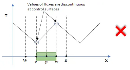
Case II : Considering a linear interpolation function which is discontinuous inside the control volume at the grid or nodal point but continous over the control surface
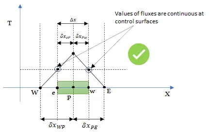
This case helps us give an insight of conserving the heat flux at the control surfaces by compromising the discontinuity inside the control volume, so that the conervation of flux is maitained at the control surface. Amount of flux entering the control surface at west end is equal to amount of flux leaving the control surafce at east end.Hence this linear function can be useful for interpolating interface data of temperature between the control syurface and grid point.
Why a linear interpolation function serves better than any higher order interpolation function ?
By intuition, a higher order interpolated function seems to be behave more accurately than linear function but in this case of control volume method, one has to be careful for selecting the higher order interpolated function.
Let us consider a quadratic interpolation function
Piecewise Quadratic Interpolation
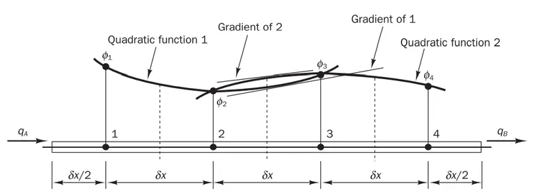
One can similarize the quadratic equation into a linear function by taking its slope and comparing it with the other curve.
From the above figure, quadratic function 1 is the curve that defines the flux entering the control surface 2 & quadratic function 2 is the function that defines the flux leaving the control suraface at point 3.
Let us find the slopes of two quadratic functions `frac{dT}[dx}` at the face of the control volume 2-3
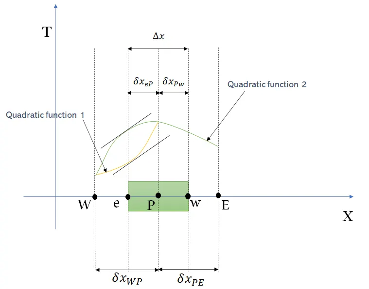
In order to conserve the flux entering at inlet control surface and exiting at the outlet control surface, the values of flux at inlet CS and outlet CS has to be the same. Therefore the slop of function 1 must be equal to the slope of function 2
NOTE : If the slope of the function 1 must be equal to the slope of other function 2, then the point 'e' must be at the point of grid/nodal points W & P for all control volumes. Therefore one must always take care of this situation before assuming higher order interpolating functions.
If interpolated without modying the slope for flux conservation, the results are no more accurate since flux at function 1 is no ore equal to flux at function 2 which violates the basic conservation of g.d.e
For Non-linear equation of Steady-State Heat conduction problem :
Non-linearity is observed when k & S are functions of T
Let us say that S(T) = 0
Assuming S to be a linear function of T
Therefore we can say that S = a + bt
Now employing the value of S into the g.d.e and integrating this over the control volume
`int_w^efrac{d}{dx}(k*frac{dt}{dx})*dx +int_w^e(a+bt)*dx) = 0`
Assuming piecewise linear 'T' assumption
`[k*frac{dt}{dx}]_e - [k*frac{dt}{dx}]_w + int_w^e (a+bT)*dx= 0`
CASE I : For constant T profile of source term
`a_P*T_P = (a_E*T_E )+(a_w*T_W) + b`
where b = `a*Deltax`
CASE II : For non-linear source term of T
Source term linearization :
Consider a non linear function of source S(T)
Ex : `S = 3 - 4T^3`
From the equation we can clearly compare that `S = S_C + S_P*T_P` , where the value of `S_P` is negative, which makes our solution to the problem a physically consistent
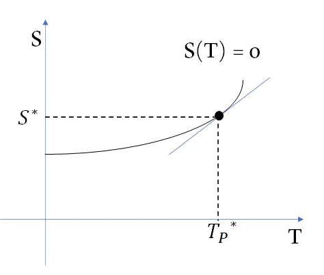
Now our motive is to convert thsi non-Linear term into linear equation
Let us represent the non-linear equation as linear by taking a tangent to the non-linear curve.
Therefore by straight lines
`y-y_1 = m*(x-x_1)`
similarly
`(S-S^star) = frac{dS}{dT}rfloor_(T_P^star) * (T - T_P^(star)) => (1)`
Now
`S = 3 - 4T^3` and
`S^star = 3-4* T_P^(3star)`
Therefore
`frac{dS}{dT}rfloor_(T_P^star) = -12*T_P^(star2)`
Substituting the values determined from above to eqn (1)
`S -(3-4T_P^(star3)) = (-12T_P^(star2))*(T-T_P^star)`
`:. S = [3+8*T_P^(3star)] -[(12T_P^(star2))*T ]`
This is the way to convert a non-linear source term into linear term
Discretization Schemes and its assement for application
1. Central Differencing Scheme (CDS)
2. Upwind Differencing Scheme (UDS)
3. Hybrid Differencing Scheme
4. Quadratic Upwind Differencing Scheme (QUICK)
5. Total Variation Diminishing (TVD)
CDS
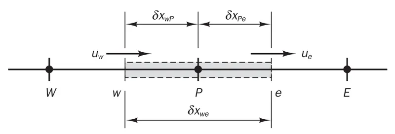
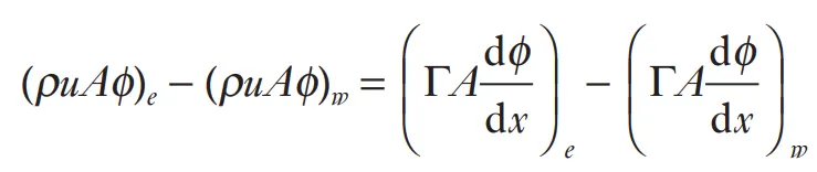
Assessment :
Conservativeness
Scheme is conservative
Boundedness
- The coefficients of the central differencing scheme satisfy the Scarborough criterion
- With aE = De − Fe/2 the convective contribution to the east coefficientis negative; if the convection dominates it is possible for aE to benegative. Given that Fw > 0 and Fe > 0 (i.e. the flow is unidirectional),for aE to be positive De and Fe must satisfy the following condition:
Fe/De = Pe < 2
If Pe is greater than 2 the east coefficient will be negative. This violates one of the requirements for boundedness and may lead to physically impossible solutions.
Transportiveness
Scheme does not recognise the direction of the flow or the strength of convection relative to diffusion. It does not possess the transportiveness property at high Pe.
Accuracy
Taylor series truncation error of the central differencing scheme is second-order
Comments on CDS Scheme & Application of usage :
It is important to note that the cell Peclet number which is a combination of fluid properties (ρ and Γ), a flow property (u) and a property of the computational grid (δx). So for given values of ρ and Γ it is only possible to satisfy condition Fe/De = Pe < 2, if the velocity is small.
Hence applicatio is mostly in diffusion-dominated low Reynolds number flows, or if the grid spacing is small. Owing to this limitation central differencing is not a suitable discretisation practice for general-purpose flow calculations.
_______________________________________________________________________________________________________________________________________________________________
UDS
For Ue, Uw > 0
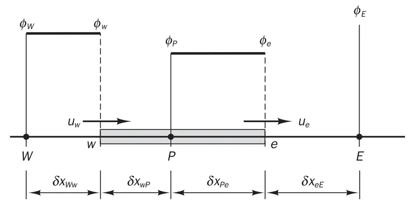
When the flow is in the positive direction, Uw > 0, Ue > 0 (Fw > 0, Fe > 0), the upwind scheme sets
`phi_w = phi_W` & `phi_e = phi_P`
The discretised equation is

Assessment :
Conservativeness
Scheme is conservative
Boundedness
The coefficients of the discretised equation are always positive and satisfy the requirements for boundedness. When the flow satisfies continuity the term (Fe − Fw) in aP is zero and gives aP = aW + aE, which is desirable for stable iterative solutions. All the coefficients are positive and the coefficient matrix is diagonally dominant, hence no ‘wiggles’
occur in the solution.
Transportiveness
The scheme accounts for the direction of the flow so transportiveness is built into the formulation.
Accuracy
The scheme is based on the backward differencing formula so the accuracy is only first-order on the basis of the Taylor series truncation error
Comments on UDS Scheme & Application of usage :
A major drawback of the scheme is that it produces erroneous results when the flow is not aligned with the grid lines. The upwind differencing scheme causes the distributions of the transported properties to become smeared in such problems. The resulting error has a diffusion-like appearance and is referred to as false diffusion.
False diffusion tends to disappear for finer grid size values
Majorly used for problems dealing with advection dominant for Pe > 2
____________________________________________________________________________________________________________________________________________________________________
Hybrid Differencing Scheme
The hybrid differencing scheme is based on a combination of central and upwind differencing schemes. The central differencing scheme, which is second-order accurate, is employed for small Peclet numbers (Pe < 2) and the upwind scheme, which is first-order accurate but accounts for transportiveness, is employed for large Peclet numbers (Pe ≥ 2)
The hybrid differencing scheme uses piecewise formulae based on the local Peclet number to evaluate the net flux through each control volume face.
Peclet number is evaluated at the face of the control volume.
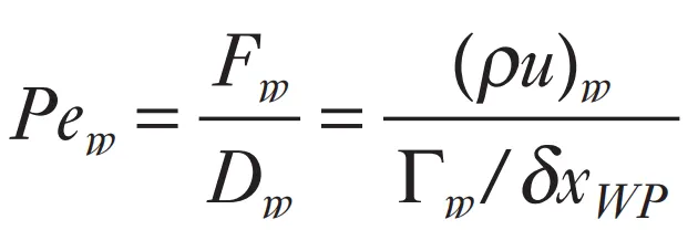
The hybrid differencing formula for the net flux per unit area through the west face is as follows:


It can be easily seen that for low Peclet numbers this is equivalent to using central differencing for the convection and diffusion terms, but when |Pe| > 2 it is equivalent to upwinding for convection and setting the diffusion to zero.
Assessment :
Conservativeness
Scheme is conservative
Boundedness
It switches to upwind differencing when central differencing produces inaccurate results at high Pe numbers. The scheme is fully conservative and since the coefficients are always positive it is unconditionally bounded
Transportiveness
The scheme satisfies transportiveness requirement by using an upwind formulation for large values of Peclet number. The scheme produces physically realistic solutions and is highly stable.
Accuracy
The scheme is based on the both central & backward differencing formula so the accuracy is only first-order on the basis of the Taylor series truncation error
Comments on Hybrid Differencing Scheme Scheme & Application of usage :
Hybrid differencing has been widely used in various CFD procedures and has proved to be very useful for predicting practical flows. The disadvantage is that the accuracy in terms of Taylor series truncation error is only first-order.
___________________________________________________________________________________________________________________________________________________________________________
Quadratic Upwind Differencing Scheme (QUICK)
The face value of `phi` is obtained from a quadratic function passing through two bracketing nodes (on each side of the face) and a node on the upstream side
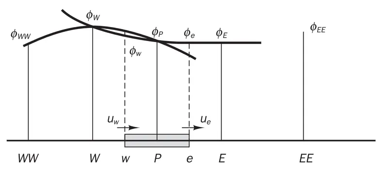
For example, when uw > 0 and ue > 0 a quadratic fit through WW, W and P is used to evaluate φw, and a further quadratic fit through W, P and E to calculate φe. For uw < 0 and ue < 0 values of φ at W, P and E are used for φw, and values at P, E and EE for φe.
It can be shown that for a uniform grid the value of φ at the cell face between two bracketing nodes i and i − 1 and upstream node i − 2 is given by the following formula
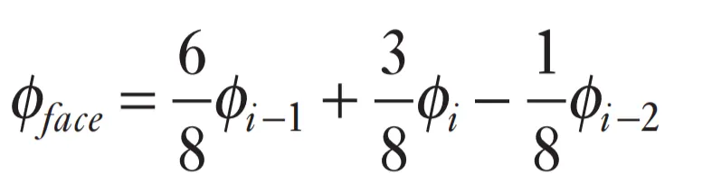
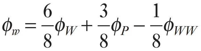
When Uw > 0, the bracketing nodes for the west face w are W and P, the upstream node is WW
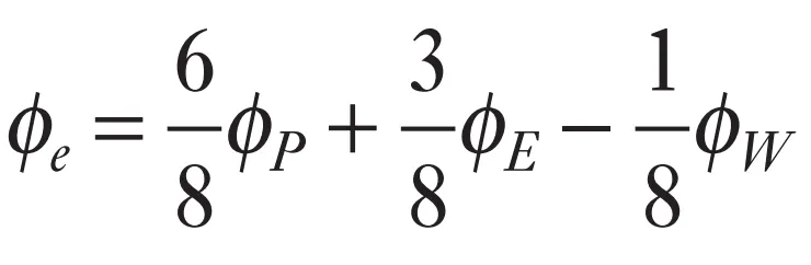
When Ue > 0, the bracketing nodes for the east face e are P and E, the upstream node is W, so
The discretised form of the one-dimensional convection– diffusion transport equation may be written as
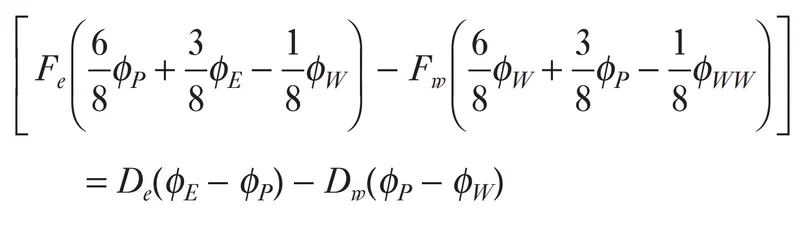
Assessment :
Conservativeness:
The scheme uses consistent quadratic profiles – the cell face values of fluxes are always calculated by quadratic interpolation between two bracketing nodes and an upstream node – and is therefore conservative.
Boundedness
If the flow field satisfies continuity the coefficient aP equals the sum of all neighbour coefficients, which is desirable for boundedness.
On the downside, the main coefficients (E and W) are not guaranteed to be positive and the coefficients aWW and aEE are negative.
For example, if
uw > 0 and ue > 0 the east coefficient becomes negative at relatively modest cell Peclet numbers (Pee = Fe/De > 8/3).
This gives rise to stability problems and unbounded solutions under certain flow conditions. Similarly the west coefficient can become negative when the flow is in the negative direction.
The QUICK scheme is therefore conditionally stable
Transportiveness
The transportiveness property is built into the scheme as the quadratic function is based on two upstream and one downstream nodal values.
Comments on QUICK Scheme & Application of usage :
The QUICK differencing scheme has greater formal accuracy than the central differencing or hybrid schemes, and it retains the upwind-weighted characteristics.
The resultant false diffusion is small, and solutions achieved with coarse grids are often considerably more accurate than those of the upwind or hybrid schemes.
___________________________________________________________________________________________________________________________________________________________________________
Flux Limiters
Flux limiters are used in numerical schemes to solve problems of highly coupled pde's. By intuition, one tends to use lower order numerical schemes for solving the g.d.e so that numerical oscillations are lower and doesn't involve unstable solutions or oscillations.
On the other hand, using higher order schemes comes up with computational cost and unnecessary computational power exploitation.
Hence, the motive behind the flux limiters is to limit the spatial derivatives near discontinuities so as to maintain the physical consistency of the problem. Highly applicapble in the formation of shock blasts, sharp peaks presence.
Flux limiters are also reffered to as slope limiters, since both are mathematically similar and physically limit the solution gradient near formation of shocks or any discontinuties
`F(u_(i+1/2)) = f^(low)(i + 1/2) - phi(r_i)(f^(low)(i+1/2) - f^(high)(i+1/2))`
`F(u_(i-1/2)) = f^(low)(i - 1/2) - phi(r_i-1)(f^(low)(i-1/2) - f^(high)(i+1/2))`
`f^(low)` - First order flux
`f^(high)` - Higher order flux
`phi(r)` - Flux Limiter function of r
where `r = [frac{u_i - u_(i-1)}{u_(i+1) - u_i}]`