Stability Analysis of Linear Systems
Stability analysis of linear systems
The linear equation to be solved is `A*X = B`
`A = [[5 ,1, 2],[-3,9,4],[1,2,-7]]` `X = [[x1],[x2],[x3]]` `B = [[10],[-14],[33]]`
`[[5 ,1, 2],[-3,9,4],[1,2,-7]]*[[x1],[x2],[x3]] = [[10],[-14],[33]]`
Values of X can be found be Iterations techniques as follows using L-U Decomposition method :
Matrix A is decomposed to its seperate diagonal matrix, lower & upper triangular matrix
Let D = diagonal matrix
L = Lower triangular marix
U = Upper triangular matrix
A = D+L+U
`[[5 ,1, 2],[-3,9,4],[1,2,-7]]` = `[[5 ,0, 0],[0,9,0],[0,0,-7]]`+`[[0 ,0, 0],[-3,0,0],[1,2,0]]`+`[[0 ,1, 2],[0,0,4],[0,0,0]]`
1. Jacobi Iteration Method :
`X_(n e w)^(Jacobi) = [B*D^-1] + [D^-1 *(-L-U)*X_(o l d)]`
Iteration Matrix : `T_(j a c) = D^-1 *(-L-U)`
2. Gauss-Seidal Iteration Method :
`X_(n e w)^(GS) = B*(L+D^-1) + [(L+D^-1) *(-U)*X_(o l d)]`
Iteration Matrix : `T_(G S) = (L+D)^-1 *(-U)`
3. SOR Iteration Method :
`X_(n e w)^(SOR) = (1- omega)*X_(o l d) + omega(X_(n e w)^(GS))`
Iteration Matrix : `(D + omega*L)^-1 + ((1-omega)*D) + (U*omega)`
Our motive is to modify the diagonal elements of Iteration matrix of each iterative solver using a magnification factor given in the data and analyse the resulting changes in Spectral Radius
To understand how to find eigen value of a matrix & its spectral radius, below is the example
Similarly we have to find the eigen values of Iteration matrix & find the spectral radius of the iteration matrix using Matlab :
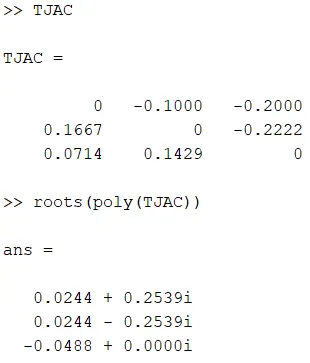
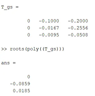
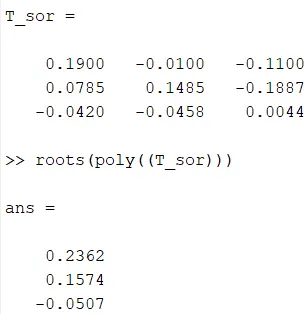
Eigen value in matlab can be found out by using poly for extracting a polynomial of Iterative matrix and then using roots to find the roots of a polynomial
Eigen Values for Iteration Matrix without using the function "eig"
Jacobi Iteration Matrix :
Gauss- Seidal Iteration Matrix :
SOR Iteration Matrix :
Matlab code to magnify diagonal matrix of usng magnifying factor :
clear all
close all
clc

%% Stability Analysis of Linear System of equations

% Defining Input Data
% For equation AX = B
A = [5 1 2; -3 9 4; 1 2 -7];               % Defining the Matrix 'A'
B = [10 -14 33];                           % Defining the Matrix 'B'
I = [1 0 0 ; 0 1 0 ; 0 0 1];               % Identity Matrix
D = diag(diag(A));                         % Diagonal Matrix is obtained by using "diag" command twice
L = (tril(A)-D);                           % Lower triangular matrix obtained by using "tril" command
U = (triu(A)-D);                           % Upper triangular matrix obtained by using "triu" command
d_mag = 0.1:0.1:2;                         % Magnification factor increasing in the rate of 0.1 units for diagonal elements
OMG = 0.9;                                 % Relaxation Factor for SOR Iterative Method

for i = 1:length(d_mag)
    D_new = D*(d_mag(i));                  % Magnifying Diagonal Matrix using magnification factor

    % Jacobi Iterative matrix

    TJAC = (inv(D_new))*(-L-U);
    [jac_iter(i),X_JAC] = jacobian_stbl(L,U,D_new,B);% Updated Iterative Matrix for magnified diagonal elements
    eig_T_JAC = roots(poly(TJAC));                   % eigen value of T_JAC can be found by converting T_JAC into polynomial "poly" and then its roots "roots"
    spctrl_rds_TJAC(i) = max(abs(eig_T_JAC));        % Finding spectral radius of T_JAC


    % G-S Iterative Matrix

    T_gs = (inv(L+D_new))*(-U);               % Updated Iterative Matrix for magnified diagonal elements
    eig_Tgs = roots(poly(T_gs));              % eigen value of T_gs can be found by converting T_JAC into polynomial "poly" and then its roots "roots"
    spctrl_rds_Tgs(i) = max(abs(eig_Tgs));    % Finding spectral radius of Tgs
    [gs_iter(i),X_GS] = gs_stbl(L,U,D_new,B);

    % SOR Iterative Matrix

    T_sor = (inv(D_new+(OMG*L)))*(((1-OMG)*D_new)-(U-OMG));               % Updated Iterative Matrix for magnified diagonal elements
    eig_Tsor = roots(poly(T_sor));           % eigen value of T_sor can be found by converting T_JAC into polynomial "poly" and then its roots "roots"
    spctrl_rds_Tsor(i) = max(abs((eig_Tsor))); % Finding spectral radius of T_sor
    [sor_iter(i),X_SOR] = sor_stbl(L,U,D_new,B,OMG);


end

figure(1)
subplot(2,1,1)
plot(d_mag,spctrl_rds_TJAC,'linewidth',1,'Marker','*')
xlabel('Diagonal Magnification');
ylabel('Spectral Radius');
title('Jacobi Iterative Method')
grid on
subplot(2,1,2)
plot(spctrl_rds_TJAC,jac_iter,'linewidth',1,'Marker','*');
xlabel('Spectral Radius');
ylabel('No of Iterations');
grid on


figure(2)
subplot(2,1,1)
plot(d_mag,spctrl_rds_Tgs,'linewidth',1,'Marker','*')
xlabel('Diagonal Magnification');
ylabel('Spectral Radius');
title('Gauss-Seidal Iterative Method')
grid on
subplot(2,1,2)
plot(spctrl_rds_Tgs,gs_iter,'linewidth',1,'Marker','*');
xlabel('Spectral Radius');
ylabel('No of Iterations');
grid on

figure(3)
subplot(2,1,1)
plot(d_mag,spctrl_rds_Tsor,'linewidth',1,'Marker','*')
xlabel('Diagonal Magnification');
ylabel('Spectral Radius');
title('SOR Iterative Method')
grid on
subplot(2,1,2)
plot(spctrl_rds_Tsor,sor_iter,'linewidth',1,'Marker','*');
xlabel('Spectral Radius');
ylabel('No of Iterations');
grid on
Function code to compute X of each iterative method :
Jacobi Iterative Method Code :
function [jac_iter,X_JAC] = jacobian_stbl(L,U,D_new,B)
xold = [0;0;0];
error = 9e9;
tol = 1e-4;
jac_iter = 1;
     while error > tol
         X_JAC = ((inv(D_new)).*B) + ((inv(D_new))*(-L-U)*xold);
         error = max(abs(X_JAC - xold));
         xold = X_JAC;
         jac_iter = jac_iter + 1 ;
     end

end
Gauss-Seidal Iterative Method Code :
function [gs_iter,X_GS] = gs_stbl(L,U,D_new,B)
xold = [0;0;0];
error = 9e9;
tol = 1e-4;
gs_iter = 1;
     while error > tol
         X_GS = ((inv(L+D_new)).*B) + ((inv(L+D_new))*(-U)*xold);
         error = max(abs(X_GS - xold));
         xold = X_GS;
         gs_iter = gs_iter + 1;
     end
end
SOR Iterative Method code :
function [sor_iter,X_SOR] = sor_stbl(L,U,D_new,B,OMG)
xold = [0;0;0];
error = 9e9;
tol = 1e-4;
sor_iter = 1;


     while error > tol
         X_SOR = (1-OMG).*(xold)+(OMG).*(((inv(L+D_new)).*B) + ((inv(L+D_new))*(-U)*xold));
         error = max(abs(X_SOR - xold));
         xold = X_SOR;
         sor_iter = sor_iter + 1;
     end
end
Observations :
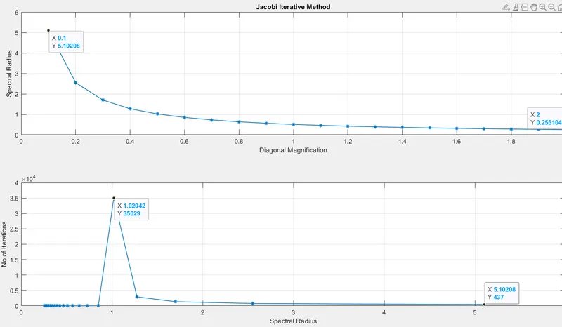
- `(rho) alpha (1/(D_m))` where `D_m` is diagonal magnification. As the magnitude of diagonal elements increases, spectral radius decreases.
- No of Iterations required to converge shoots up for Spectral radius >1
- Total no of Iterations required when spectral radius >1 is nearly equal to 35000
1. Jacobi Iterative Method :
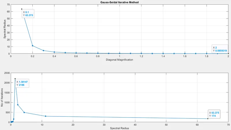
2. Gauss-Seidal Iterative Method :
- `(rho) alpha (1/(D_m))` where `D_m` is diagonal magnification. As the magnitude of diagonal elements increases, spectral radius decreases.
- No of Iterations required to converge shoots up for Spectral radius >1
- Total no of Iterations required when spectral radius >1 is nearly equal to 2300 which is 15 times less than Jacobi Iterative technique
3. SOR Iterative Method :
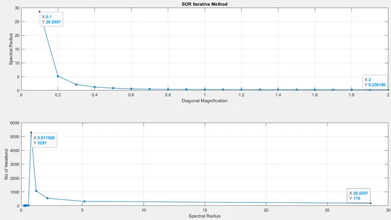
- `(rho) alpha (1/(D_m))` where `D_m` is diagonal magnification. As the magnitude of diagonal elements increases, spectral radius decreases.
- No of Iterations required to converge shoots up for Spectral radius >1
- Total no of Iterations required when spectral radius >1 is nearly equal to 5500 which is 5 to 6 times less than Jacobi Iterative technique.
NOTE : Due to non selection of optimised omega value, no of iterations is shooting up ore than Gauss-Seidal Technique
Solution for Q1 :
Convergence rate of the solution is dependant on 2 things
- Diagonally Dominant matrix
- Magnitude of Spectral Radius
1. Diagonally Dominanat Matrix :
`Y =[[a11, a12,a13],[a21,a22,a23],[a31,a32,a33]]`
then for matrix Y to be diagonally dominant
`|a_11| > |a_12+a_13|`
`|a_22| > |a_21+a_23|`
`|a_33| > |a_31+a_32|`
2.
`G = [[5 ,1, 2],[-3,9,4],[1,2,-7]]`
To find the eigen values of G :
`|G-lamdaI| = 0`
where I is the identity vector `I = [[1 ,0, 0],[0,1,0],[0,0,1]]`
`|[5-lamda,1,2],[-3,9-lamda,4],[1,2,-7-lamda]| = 0`
`lamda_1 = 8.4900`
`lamda_2 = 6.1763`
`lamda_3 = -7.663`
Spectral Radius of G i.e `rho(G) = max|(lamda)|`
`rho(A) = 8.4900`
But for a faster convergence of problem spectral radius for a solution has to be < 1
Solution for Q2 :
Diagonal Dominance :
Diagonally Dominanat Matrix :
`Y =[[a11, a12,a13],[a21,a22,a23],[a31,a32,a33]]`
then for matrix Y to be diagonally dominant
`|a_11| > |a_12+a_13|`
`|a_22| > |a_21+a_23|`
`|a_33| > |a_31+a_32|`
Relationship between diagonal dominance and Spectral radius is an inverse relation i.e the solution tends to converge faster for high diagonal dominant elements
Plot below is the proof of this relation :