Week 5 - Turbulence modelling challenge
Aim:
To perform a 3-D Turbulant simulation on the given model. And to understand the various turbualnce models present.
Objective:
- To simulate for the given flow conditions for the golf ball and visuvalize and analyse the wake region around it.
- To understand and explain the various turbulance model available.
Introduction:
Dynamics of Golf Ball:
When a golf ball is hit, the impact, which lasts less than a second determines the ball's velocity, launch angle and spin rate, all of which influence its trajecctory and its behavior when it hits the ground. A ball moving through air experiences two major aerodynamic forces, lift and drag. Dimpled balls fly farther than non-dimpled balls due to the combination of these two effects. The aerodynamics of golf balls is considerably more complex than that of many other spherical balls. The surface roughness in the form of dimples intensifies the level of complexity and three-dimensionality of air flow around the golf ball.
First, the dimples on the surface of a golf ball cause the boundary layer on the upstream side of the ball to transition from laminar to turbulent. The turbulent boundary layer is able to remain attached to the surface of the ball much longer than a laminar boundary with fewer eddies and so creates a narrower low-pressure wake and hence less pressure drag. The reduction in pressure drag causes the ball to travel further.
Second, the backspin generates lift by deforming the airflow around the ball, in a similar manner to an airplane wing. This is called the Magnus effect. The dimples on a golf ball deform the air around the ball quickly causing a turbulent airflow that results in more Magnus lift than a smooth ball would experience. A backspinning ball experiences an upward lift force which makes it fly higher and longer than a ball without spin.
To keep the aerodynamics optimal, the golf ball needs to be clean, including all dimples. The two major drag associated in a body is pressure and friction drag, the pressure drag occurs when there is a pressure difference between front and at the back of the body and it is significant in bluff bodies, it is an object that due to its shape causes separated flow over most of its surface. The friction drag occurs due to the friction due to flow over rough surface and it is common in Streamline bodies such as aerofoils.
Initially the golf balls were smooth and were not able to travell longer distance.The streamline flow on the surface of the smooth golf ball, then, will also result in a higher drag because the low pressure region generated will exceed the high pressure region. But soon the introduction of dimples to create a rough surface and to convert it to a turbulant flow gave the requires results by causing delayed flow seperation and less drag due to swriling air.
In case of a dimpled golf ball, the streamline flow remains attached to the surface of the ball for a much longer period thereby reducing the low pressure area behind the ball and causing much less drag thereby enabling the ball to travel farther. Moreover, the dimples generate lift when there is significant backspin on the ball as it is sailing through air.
Critical Number:
Critical number reffers to the reynolds number for a paticular model for which the flow becomes turbulant in nature.
To understand better about the golf ball dynamics we must first know about different types of flows present.
Laminar Flow:
Laminar flow, also called streamline flow, type of fluid flow in which the fluid travels smoothly or in regular paths. The flow will be laminar when the reynolds number is less than 2200. In laminar flow the viscous effects are dominant and properties such as velocity and pressure are constant.
Turbulant Flow:
Turbulant flows occur when the reynolds number is greater than the critical reynolds number.In this case the the inertial forces dominate and leads to formation of instablities and vortices.
Transient Flows:
The transition from laminar to turbulant flow is what catoragrised as transition flow. There will be significant f=effects of both viscous and inertial forces.
Since the turbulant flows are instable and contniously changes with time and are unpredictible, it is hard to predict and study the formation of turbulant flows. With the use of genarated vortices in this flows scientist studied the coherent structures in flow to better modelling. By this way we were able to better modulate for the turbulant flows.
In turbulant flows there will be formation of vortices or eddies. With respect to reynolds number and the surface over the fluid flows the size of eddies formed will be changed, the bigger eddies could break beyond certain point and form smalled eddies or the smaller eddies could combine and form bigger eddies. To account and follow each eddies the mesh or grid size has to be small and perfect size so not to have a large computational time. The models developed for this are of three types,
DNS -
Direct Numerical Simulation solves for a small eddie formations. To calculate the perfect grid size to calculate the navier stoke's Equation the relation is given as,
`eta propto 1/((Re)^(3/4))`
Therefore the grid size must be smaller than '`eta`'. To calculate the number of elements used in this model,
N= Total volume of all elements / Volume of the single element
`N propto (Re)^ (9/4)`
The reason why the DNS is not feasible when we consider Kolmogrov, scale is for turbulant flow the reynolds number is very high and therefore the grid size `eta` becomes very small which leads to high computational time. Simillarly for the number of elements will be very large in number for a given 3-D simulation. So this model is only preffered for 2-D applications.
LES -
Large Eddy Simulation are used for paticularly resolving larger eddies as they are less accurate for smaller eddies. The number of elements is also less as they are dependent on the characteristic length and velocity.
RANS -
Reynolds Averaged Navier Stoke's Equation is a common model used in Fluent and is less expensive for industrial cases. In this method the Navier Stoke's equation is decomposed and solved. That is the contnuity,momentum,and energy equations are averaged. This gives rise to reynolds stress terms and to model for these terms is important to get accurate results. So, further models are developed to solve these stresss terms.
The models developed to account for the reynolds stresses developed after solving Navier Stoke's equation for compressible flows.
First Order Models :
The first order model uses PDE's of first orded to find the turbulant viscosity.
Zero Equation Model -
This model does not use the PDE to solve for the turbulant viscosity, tey fail to account for the transient behavoiur of turbulant viscosity. They solve for turbulant viscosity using Mixing length model. The Eddy vidcosity model are similar to two Kolmorgov models.
One Equation Model -
Also known as Spalart Allmaras model uses PDE's to solve the Turbulant Kinetic Energy to solve the Turbulant Viscosity.The Spalart–Allmaras model was designed specifically for aerospace applications involving wall-bounded flows and has been shown to give good results for boundary layers subjected to adverse pressure gradients. It is also gaining popularity in turbomachinery applications. Because there is only one dynamic differential equation to solve, it is computationally much simpler than a DNS approach. The turbulant viscosity is then solved by substuting in RANS model.
Two Equation Model -
This model uses two equations to solve the ,
- Turbulent Kinetic Energy and Turbulant Dissipation rate
- Turbulent Kinetic Energy and Specific Dissipation rate
These two are the most commonly used models to solve industrial problems. The two equation model are of types,
K-epsilon Model :
K epsilon is best suited for flow away from the wall, say free surface flow region.
Standard K-epsilon Model -
They are highly accurate in capturing the near wall changes in the model, the solution unlike other models converges quickly and therafore needed very less memory for solving any model. Since they are effective in computing for high turbulant flows around complex bodies and attached flows they are widely preffered in industries. They are not recommended when solving for seperated flows.
Realizable K-epsilon Model -
In this model modfies the epsilon equation to solve for additional reynolds stress trems. As a result it mainly gives improved predictions for the spreading rate of jets, a superior ability to capture the mean flow of complex structures and for flows involving rotation, boundary layers under strong adverse pressure gradients, separation and re circulation.
Renormalized Group (RNG) Model -
They uses the renormalized gropu theory to improve the epsilon equation. To account for the effects of smaller scales of motion. In the standard k-epsilon model the eddy viscosity is determined from a single turbulence length scale, so the calculated turbulent diffusion is that which occurs only at the specified scale, whereas in reality all scales of motion will contribute to the turbulent diffusion. The RNG approach, which is a mathematical technique that can be used to derive a turbulence model similar to the k-epsilon, results in a modified form of the epsilon equation which attempts to account for the different scales of motion through changes to the production term. It uses emperical relations to find the Prandel Number.
K-omega Model :
The k-omega model is best suited for near the wall flow region, where adverse pressure gradient is developed. They don't require to define the wall functions as it is already defined in this model.
Standard K-omega Model -
The standard k−ω model is a low Re model, it can be used for flows with low Reynolds number where the boundary layer is relatively thick and the viscous sublayer can be resolved.
Thus, the standard k−ω model is best used for near-wall treatment. Other advantages include a superior performance for complex boundary layer flows under adverse pressure gradients and separations like in external aerodynamics and turbomachinery. On the contrary, this model has also shown to predict excessive and early separations.
SST K-omega Model -
The SST formulation switches to a k-epsilon behavior in the free-stream, which avoids the k−ω problem of being sensitive to the inlet free-stream turbulence properties. The k−ω SST model provides a better prediction of flow separation than most RANS models and also accounts for its good behavior in adverse pressure gradients. They use a blending function for transition from standard model to higher reynolds model away from the wall. It is the most commonly used model in the industry given its high accuracy to expense ratio.
Second Order Models :
This model solves Reynolds transport equations to solve reynolds stress terms. Since they solve the PDE's of second order they provide accurate results, they are widely used to solve for 3-D simulation models. They are highely responsive to boundary conditions. They are computationally expensive.
Algebric Stress Model -
It is developed from model dynamics equation. In the first, the transport of the turbulent stresses is assumed proportional to the turbulent kinetic energy; while in the second, convective and diffusive effects are assumed to be negligible.
Reynolds Stress Model -
The Reynolds Stress Models (RSM), also known as the Reynolds Stress Transport Models, are higher level turbulence closures and represent the most complete classical turbulence model. The method of closure employed is usually called a Second Order Closure
Kolmogorov's Scale :
Kolmogorov's Scale are the smallest scales in turbulant flow. At the Kolmogorov scale, viscosity dominates and the turbulent kinetic energy is dissipated into heat. They are used to determine the size of the eddies formed in a turbulance model. ANd from the size it is calculated how much energy does each eddies have. Further these formed eddies gould be dispersed into smaller eddies or smaller eddies could combine to form larger eddies.
To determine the size to energy dissipation of eddies the below relation is arrived,
For larger eddies `propto (L/(U infty))`
For smaller eddies `propto (L /(Re)^(3/4))`
| Kolmogorov length scale |  |
| Kolmogorov time scale |  |
where `varepsilon`is the average rate of dissipation of turbulance kinetic energyper unit mass, and `upsilon` is the kinematic viscosity of the fluid.
Procedure :
First we open the model in design modular and visuvalize the geomentry and creat an volume enclosure around the golf ball for the fluid-solid interaction.
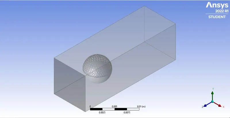
We then open the meshing solver and generate the mesh for the size of 3.5 mm for the enclosed region and 3 mm for the golf ball.
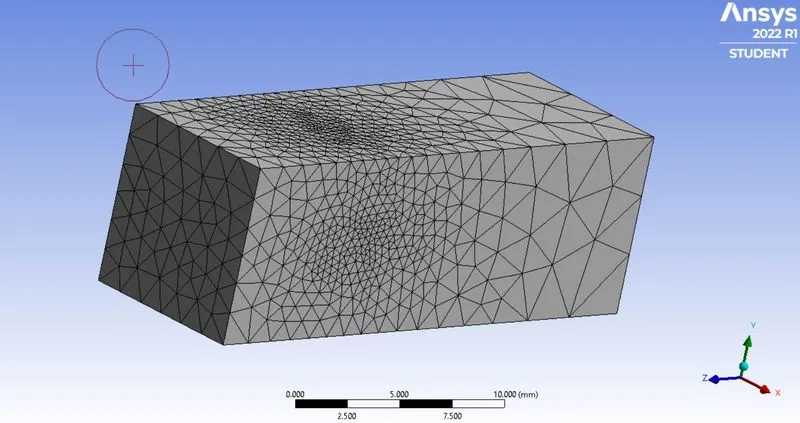
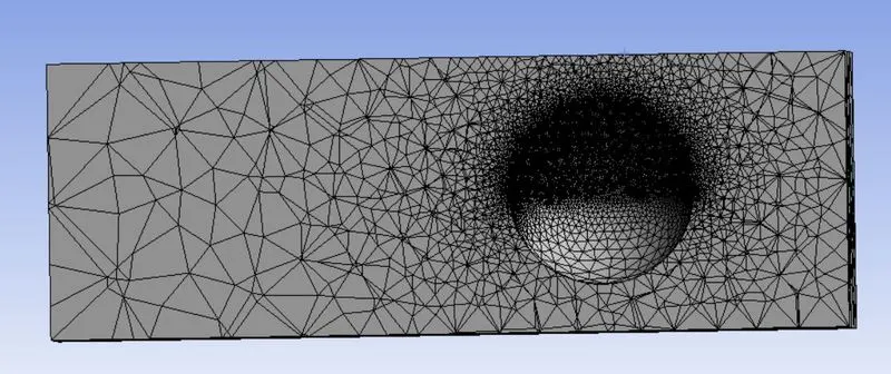
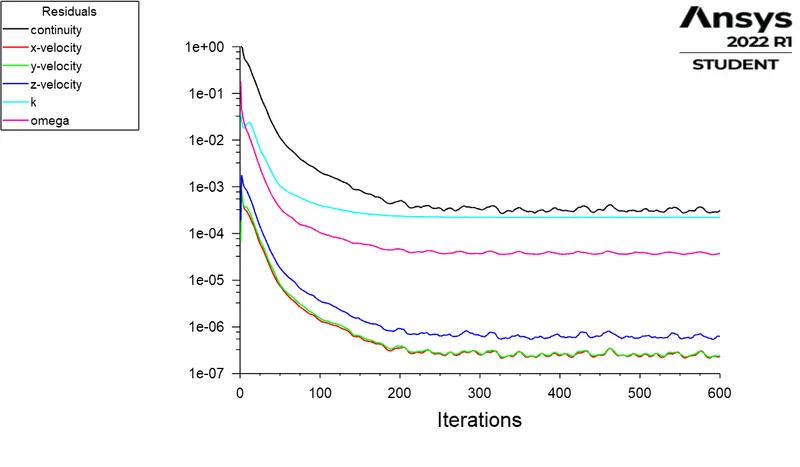
Then in solution setup we define it as pressure based solver and choose the k-`omega` SST model for solving, as this is a low reynolds number problem and we need to also observe the neaw wall changes. We give the inlet velocity as 60 m/s. We then initialize the solution and run for 600 iterations.
For results we observe the velocity and pressure contour.
Results :
Resuidal -
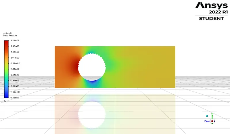
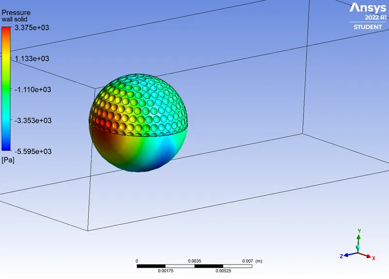
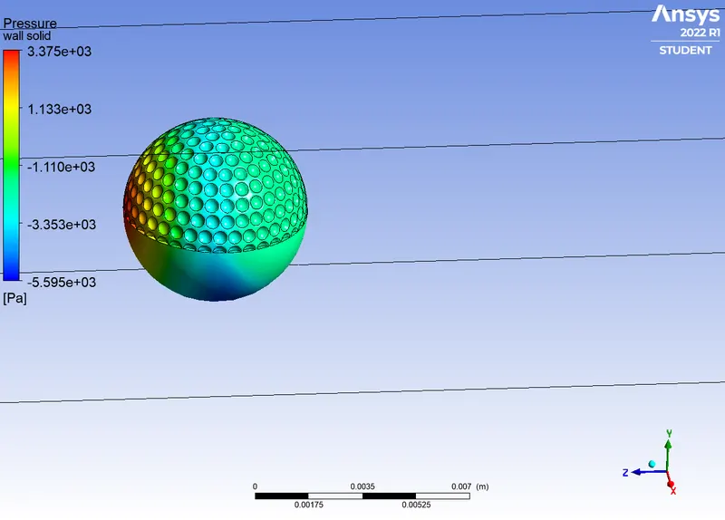
Pressure Contour -
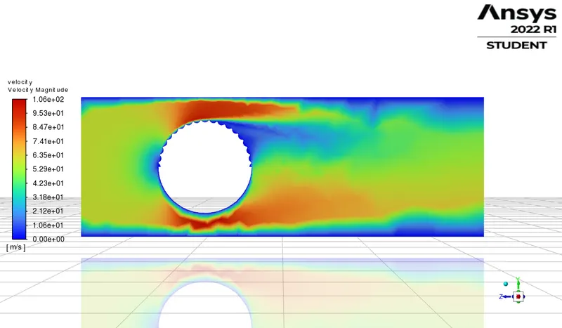
Velocity Countour -
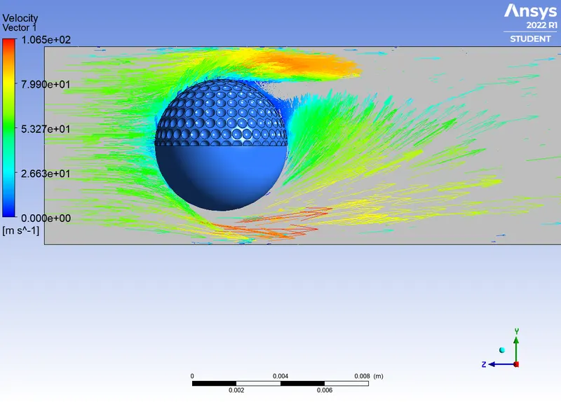
Velocity Vector -
Conclusion :
From the contour we can visuvalize that the pressure is high in front and low at the back this creates a pressure drag on the ball, Therefore this genarates the spin and the ball swirls. Also at the bottom there exist a negative pressure region and the probable spin on the ball will be top to bottom this gives the golf ball to travell longer at the same time create more lift.
With the velocity profile we can see thare is a two flow seperation region one at the top and one at the bottom. The given geomentry is the bottom surface is smoth an the top surface have dimples. From the theory discussed above the dimples converts laminar flow into turbulant flow and causes delayed flow seperation. We can see that the top flow is turbulant and causes disturbance and with the generated energy there is a delayed seperation and the wake region of low pressure is formed just behind the seperation point, this will suck air and generate spin. And due to smooth surface the bottom surface have early flow seperation and as the surface is smooth the velocity magnitude at the bottom is very high as that of above. Therefore the ball will spin anti-clockwiese direction / Top spin.