Week 5.1 - Mid term project - Solving the steady and unsteady 2D heat conduction problem
The heat conduction is re[resented as a partial differentiation equation that shows the heat progression over time.The 2-D heat conduction equation is given by ,
`(delT)/(delt) +alpha ((del^2T)/(delx^2) +(del^2T)/(dely^2)) =0`
where '`alpha`' is Thermal diffusivative term.
The time derivative term '`(delT)/(delt)`' will be 0 under steady state condition.
After discretization the steady state equation will be
`Tp = 1/k((T(i-1,j)+T(i+1,j))/(Deltax^2)) +1/k ((T (i,j-1)+T(i,j+1))/(Deltay^2))`
where k=`2*((Deltax^2 +Deltay^2)/(Deltax^2*Deltay^2))`
Since all the terms are calculated at 'n' which is known we can use any of the iterative solvers to compute itrative solvers to compute.
1.Jacobie
2.Gauss-Seidal
3.Successive over-relaxation
For Jacobi equation the The temperature value computed for previous iteration such as '`T(i-1,j)`' , ' T (i,j-1)`' , '`T(i+1,j)`' and '`T(i,j+1)`'will take value of T from Told(the temperature at previous point).
Simallarly For Gauss-Seidal the Temperature of terms '`T(i-1,j)`' and ' T (i,j-1)`' will not take the Told value which is computed for previous point.
For SOR the equation is,
`Tp^(n+1) = T(i,j)(1-alpha) + alpha( T Gauss (or) Tjacobi)`
Where,
`alpha >1 ,Over Relaxation`
`alpha < 1 ,Under Relaxation`
For Transient Flow ,we can compute using two equations on is at 'n'th position and other at 'n+1' position and they are called as Explicit and Implicit solutions respectively.
Explicit solution:
`Tp^(n+1) =T(i,j) + K1*((T(i-1,j) -2(i,j)+T(i+1,j)) +K2*(T(i,j-1) -2(i,j)+T(i,j+1))`
We will include a time loop for solving the equation. Where,
K1=`(alpha (Deltat))/(Deltax^2)`
K2=`(alpha (Deltat))/(Deltay^2)`
In case of Explicit diffusive case `K1+K2 <= 0.5` else the solution will be unstable.
Implicit solution:
`Tp^(n+1) =(T(i,j) + K1*(T(i-1,j) +T(i+1,j))+K2*(T(i,j-1)+T(i,j+1)) )/(1+2*K1+2*K2)`
We can then solve the exuation by Applying any of the three Iterative Solvers as done for steady state condition. In addition we have to introduce the Time step for each iteration.
Procedure:
1. We first define the initail conditions including the temperature at each faces.
2. We create a mesh grid for converting the 1-D array x& y of length nx,ny respectively into 2-D matrix for ploting.
3. We give error and threshold value so that the iteration stops when the error is less than threshold value.
4. We generate a for loop for solving the equation and update the Told value at the end of convergece loop.
5. Then we plot the Temperature contour for each equation, display the total simulation time and No.of iterations.
6. For transient flows we add a time loop for defining each time step.
7. For Transient flow equations we plot the graph inside the time loop.
clear all
close all
clc

%Defining the Input paramaters
nx=11;
ny=11;
x=linspace(0,1,nx);
y=linspace(0,1,ny);
dx=x(2)-x(1);
dy=y(2)-y(1);
k=2*(dx^2+dy^2)/(dx*dy)^2;

%defining the Temperature on four boundarys
T= 300*ones(nx,ny);
T(1, :) = 600;
T(nx, :) = 900;
T(: ,1) = 400;
T(: ,ny) = 800;
T(1,1) = 500;
T(1,ny)= 700;
T(nx,1)= 650;
T(nx,ny)= 850;
Told= T;
Tprv=T;


Iterative= input('Enter the number(1-3) to choose Iteretive Method: ')
[xx,yy]=meshgrid(x,y);
error= 9e9;
threshold= 1e-4;

%Jacobi
if  Iterative == 1
tic %stopwatch
Jacobiite=1;
while(error>threshold)
    for i=2:nx-1
        for j=2:ny-1
            Term1= (Told(i-1,j)+ Told(i+1,j))/dx^2;
            Term2= (Told(i,j-1)+ Told(i,j+1))/dy^2;
            T(i,j)= (1/k)*(Term1 + Term2);
        end
    end
    error=max(max(abs(Told-T)));
    Told=T;
    figure(1)
    contourf(xx,yy,T,'ShowText','on');
    colormap jet
    colorbar
    xlabel('space')
    ylabel('Temperature')
   Jacobiite=Jacobiite + 1 %Iterating
end
time=toc
end

%gauss-Seidal Method
if  Iterative == 2
tic
Gaussite=1;
while(error>threshold)
    for i=2:nx-1
    for j=2:ny-1
        Term1= (T(i-1,j)+ Told(i+1,j))/dx^2;
        Term2= (T(i,j-1)+ Told(i,j+1))/dy^2;
        T(i,j)= (1/k)* (Term1 + Term2);
    end
    end
    error=max(max(abs(Told-T)))
    Told=T;
    figure(1)
    contourf(xx,yy,T,'ShowText','on');
    colormap jet
    colorbar
    xlabel('space')
    ylabel('Temperature')
    Gaussite=Gaussite + 1

end
time=toc
end

%SOR
if  Iterative == 3
tic
SORite=1;
while(error>threshold)
    for i=2:nx-1
    for j=2:ny-1
        w= 1.2;
        Term1= (T(i-1,j)+ Told(i+1,j))/dx^2;
        Term2= (T(i,j-1)+ Told(i,j+1))/dy^2;
        Tgs= (1/k)* (Term1 + Term2);
        T(i,j)= Told(i,j) *(1-w)+ w*(Tgs);
    end
    end
    error=max(max(abs(Told-T)))
    Told=T;
    SORite=SORite + 1
    figure(1)
    contourf(xx,yy,T,'ShowText','on');
    colormap jet
    colorbar
    xlabel('space')
    ylabel('Temperature')
end
time=toc
end
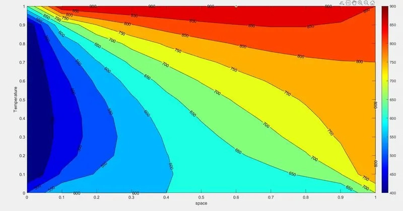
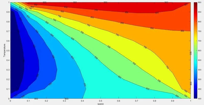
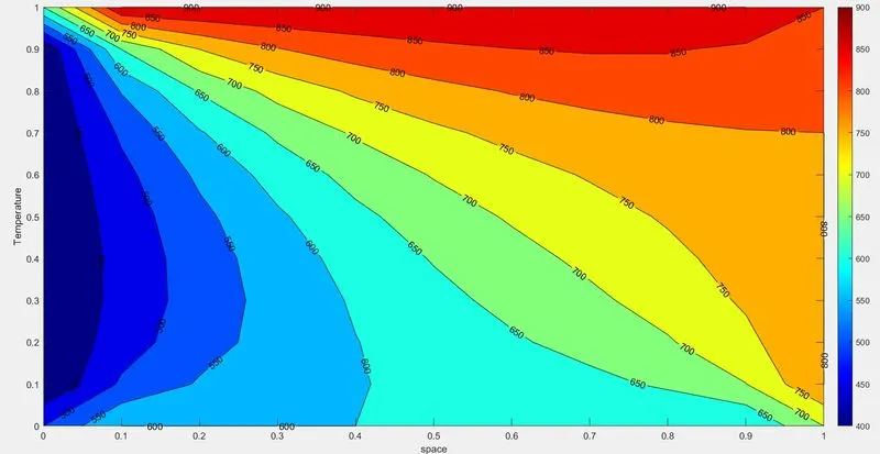
Plot :
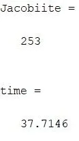
Jacobi:
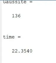
Gauss Seidel:
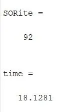
SOR:
Transient Flow:
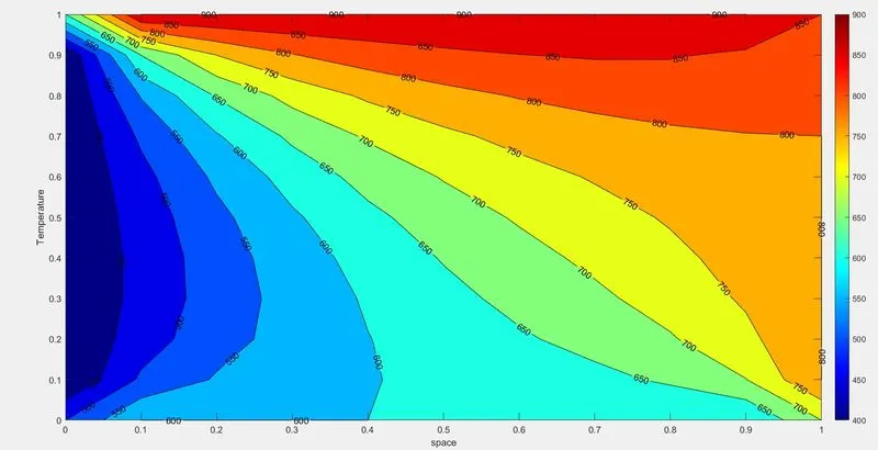
Explicit Method :
clear all
close all
clc


%Transient flow
 %Explicit function
nx=11;
ny=11;
x=linspace(0,1,nx);
y=linspace(0,1,ny);
dx=x(2)-x(1);
dy=y(2)-y(1);
k=2*(dx^2+dy^2)/(dx*dy)^2;

T= 300*ones(nx,ny);
T(1, :) = 600;
T(nx, :) = 900;
T(: ,1) = 400;
T(: ,ny) = 800;
T(1,1) = 500;
T(1,ny)= 700;
T(nx,1)= 650;
T(nx,ny)= 850;
Told= T;
[xx,yy]=meshgrid(x,y);
 a=0.25;
 dt=0.01;
 k1= a*dt/dx^2;
 k2= a*dt/dy^2;
 threshold=1e-4;

 tic
  Transjacobiite=1;
for nt=1:1400
    error=9e9;
    while (error>threshold)
        for i=2:nx-1
        for j=2:ny-1
            Term1= Told(i-1,j)-(2*Told(i,j))+ Told(i+1,j);
            Term2= Told(i,j-1)-(2*Told(i,j))+ Told(i,j+1);
            T(i,j)= T(i,j)+k1*(Term1)+k2*(Term2);
        end
        end
        error=max(max(abs(Told-T)))
        Told=T;
        Transjacobiite=Transjacobiite + 1
    end
end
figure(1)
contourf(xx,yy,T,'ShowText','on');
colormap jet
colorbar
xlabel('space')
ylabel('Temperature')
time=toc
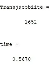
Plot and Result:
Implicit :
clear all
close all
clc
nx=11;
ny=11;
x=linspace(0,1,nx);
y=linspace(0,1,ny);
dx=x(2)-x(1);
dy=y(2)-y(1);
k=2*(dx^2+dy^2)/(dx*dy)^2;

T= 300*ones(nx,ny);
T(1, :) = 600;
T(nx, :) = 900;
T(: ,1) = 400;
T(: ,ny) = 800;
T(1,1) = 500;
T(1,ny)= 700;
T(nx,1)= 650;
T(nx,ny)= 850;
Told= T;
Tprv=T;


%Transient Flow
%Implicit
solver3=input("Enter the number(7-9) to solve for inplicit method ")
[xx,yy]=meshgrid(x,y);
threshold= 1e-4;

if solver3 == 7
    a= 1.4;
    dt=0.01;
    k1= a*dt/dx^2;
    k2= a*dt/dy^2;
    tic
     TIjacobiite=1;
    for nt= 1:1400
        error= 9e9;
        while(error>threshold)
            for i= 2:nx-1
            for j= 2:ny-1
                term1= 1/ (1+2*k1+2*k2);
                term2= k1*term1;
                term3= k2*term1;
                M= (Told(i+1,j)+Told(i-1,j));
                N= (Told(i,j+1)+Told(i,j-1));
                T(i,j)=Tprv(i,j)*term1+ term2*M + term3*N;
            end
            end
            error=max(max(abs(Told-T)))
            Told=T;
            TIjacobiite=TIjacobiite+1
        end
          Tprv=T;
    end
           figure(1)
        contourf(xx,yy,T,'ShowText','on');
        colormap jet
        colorbar
        xlabel('space')
        ylabel('Temperature')

end
 time=toc

%Gauss
if solver3 == 8
    a= 0.25;
    dt=0.01;
    k1= a*dt/dx^2;
    k2= a*dt/dy^2;
    tic
    TIgsite=1;
    for nt= 1:1400
        error= 9e9;
        while(error>threshold)
            for i= 2:nx-1
            for j= 2:ny-1
                term1= 1/ (1+2*k1+2*k2);
                term2= k1*term1;
                term3= k2*term1;
                M= (T(i+1,j)+Told(i-1,j));
                N= (T(i,j+1)+Told(i,j-1));
                T(i,j)=Tprv(i,j)*term1+ term2*M + term3*N;
            end
            end
            error=max(max(abs(Told-T)))
            Told=T;
            TIgsite=TIgsite+1
        end
          Tprv=T;

    end
     figure(1)
        contourf(xx,yy,T,'ShowText','on');
        colormap jet
        colorbar
        xlabel('space')
        ylabel('Temperature')


end
time=toc


if solver3 == 9
    a= 0.25;
    dt=0.01;
    k1= a*dt/dx^2;
    k2= a*dt/dy^2;
    tic
    TIsorite=1;
    for nt= 1:1400
        error= 9e9;
        while(error>threshold)
            for i= 2:nx-1
            for j= 2:ny-1
                term1= 1/ (1+2*k1+2*k2);
                term2= k1*term1;
                term3= k2*term1;
                w= 1.2;
                M= (T(i+1,j)+Told(i-1,j));
                N= (T(i,j+1)+Told(i,j-1));
                T(i,j)=(T(i,j)*(1-w))+(Tprv(i,j)*term1+ term2*M + term3*N)*w;
            end
            end
            error=max(max(abs(Told-T)))
            Told=T;
             TIsorite=TIsorite+1
        end
          Tprv=T;

    end
      figure(1)
        contourf(xx,yy,T,'ShowText','on');
        colormap jet
        colorbar
        xlabel('space')
        ylabel('Temperature')


end
time=toc
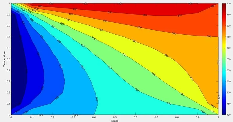
Plot and Result:
Jacobi:
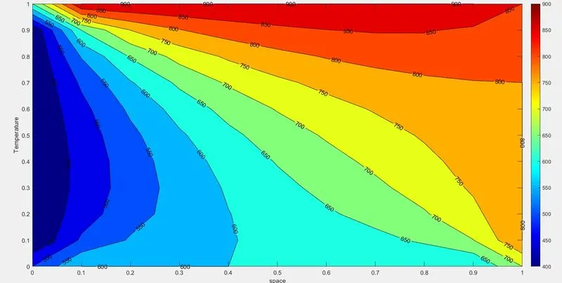
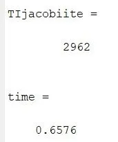
Gauss-Seidel:
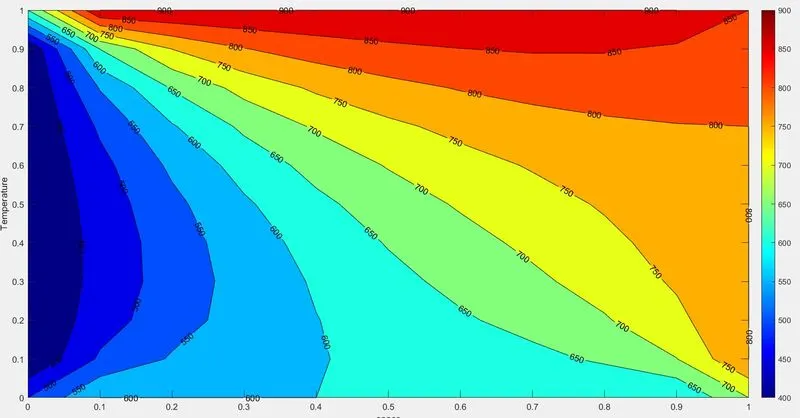
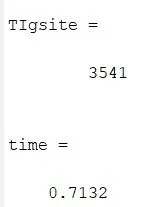
SOR:
Conclusion:
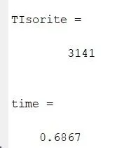
From the above results we can inffer that the among total time taken for computing steady state equation the SOR mathod is faster and requires less number of iterations than others. This is because the term `alpha` where we defined it to be over realxing.
When compared to Explicit vs Implicit solution
Explicit solution is easy to solve since solving the matrix invertion is simple and straight forward. But we have to watchout sum of CFLx and CFLy (K1+K2) terms should be `<=` 0.5. Whereas solving the invertion of implicit matrix is complex and requires iterative solvers. Theoritically the total solving time is increases in the order of SOR<Gauss<Jacobi.