Week 11- Broadband Noise modelling over Ahmed body

Aim :

To simulate for the given ahmed body and study the acoustic field around it.

Objective :

1. Describe Ahmed's body and its importance.
2. Setup the domain and setup assuming body is travelling at 110 kmph
3. Run the setup till convergence and plot for static pressure and coefficient of drag and lift to check for convergence
4. Turn on Broadband- modelling and detail the acoustic field study over Ahmed body.

Introduction :

Ahmed Body -

Ahmed body is a simplified model of a car developed to study drag force and its importance. The aerodynamic properties of a car determines the ride comfort ,stablity,and performance of a car,due to the effect of drag force sourrounding the body it creates a low pressure region at the rear end of a car called as wake region. The body can be named into three regions the front round part, a rectangular middle part and a slanting rear part. Since higher drag force could lead to more fuel consumprion,this simple model helps in designing a more suitable car to overcome the drag force. Therefore this model serves as a benchmark design for developing a car.

The different results such as drag and lift force co-efficient,velocity and pressure changes, visulising the vortices and wake regions developed can give the designers ideas to of where this points and regions so that they could introduce new designs to reduce it. The number of different studies carrier out using this model made it more powerful model as still an aerodynamic designer uses the exprimental datas of Ahmed body under wind tunnel testing to validate for their computational devloped models. As the majour flow around the body is turbulant flow either of k-epsilon or k-omega model is used to compute the results. The rear slant part is has a critical angle of 30°, the significant of this angle is immportant as this is responsible for creating the wake region at the rear end. At first hand the wake region is due to a phenemenon called as Flow Seperation that occurs at the very tip of a body,here it is the rear part. So, if the slant angle is greater it results in flow seperation and leads to creation of wake region and eventually increasing the drag-force. And for angle less than that the a counter vortices occurs which reduces the flow seperation.

Aero Acoustics -

Aeroacoustics is a branch of acoustics that studies noise generation via either turbulant fluid motion or aerodynamics forces interacting with surfaces. Noise generation can also be associated with periodically varying flows. Sound waves are generally pressure waves,therefore sound waves are mesaured as a disturbance in pressure. Classical wave equation governs the acoustic phenomeon, to computationally solve these equations there are two majour approches Direct and Hybrid method.

DNM - This method is used for unsteady turbulant flow and they are computationally expensive but can arrive at a solution faster. They use Lighthills analogy to solve the renyolds stress terms in the acoustic governing equation.

Hybrid - This approach can be used for both steady and unsteady models. The steady approach solved using RANS model and uses Broadband solver to solve and find the acoustic sources around the body. While the unsteady approach uses either of DNS/LES/URANS model and solves the acoustic phenomeon using Fowcs Williams-Hawkings solver.

Broadband Solver -

In many practical applications involving turbulent flows, noise does not have any distinct tones, and the sound energy is continuously distributed over a broad range of frequencies. In those situations involving broadband noise, statistical turbulence quantities readily computable from RANS equations can be utilized, in conjunction with semi-empirical correlations and Lighthill's acoustic analogy, to shed some light on the source of broadband noise. This model are found to be effective tools in screening turbo machine system with higher noise levels and identifying components or surfaces with high noise generation.

Procedure :

Since the two enclosures overlap ecahother ,this would result in creating mesh inside the ahmed body and we dont want this as the flow is external. We use the interference option to extrude the interfered region from the model. And we have to enable the share option to allow the enclosure to share properties. Since the entire body is perfectly symmetry we use split body to split out the other identical half from the model. This way we can refine even better and obtain more elements for accurate results. The second enclosure is created to study the wake characteristics more precisely with more mesh refinement the dimention of this enclosure is given based on the size of the wake region created.

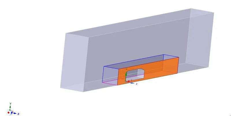
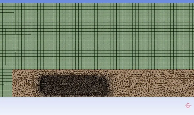
We mesh the two enclosures with different mesh sizes for better capturing of results. Then since it is an external flow over the body we need to capture the changes near the oundary layer we create inflation layer near the boundary with total thickness option and create 6 layers of inflation. The total thickness of the inflation layer is set to 8.33428 mm.

Then we open the solution setup where we define the model as steady state pressure based solver. Since for broadband model we require to select RANS model we choose k-`epsilon` standard model with enhanced wall treatment as it as an external flow over solid surface. Then under acoustic model we enable the broadband model.

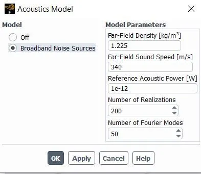
We then set the inlet boundary condition as velocity inlet of magnitude 110 m/s. We plot for lift and drag co-efficient then plot static pressure to check for convergence. We run the iteration for 500.

Results :

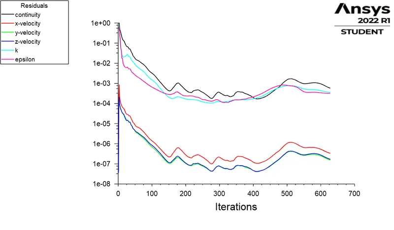
Resuidal -

Drag Co-efficient -

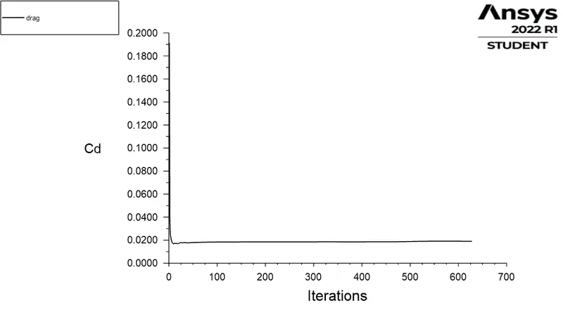
Average Drag Co-Efficient = 0.0190

Lift Co-efficient -

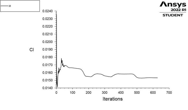
Average Lift Co-Efficient - 0.0153

Pressure -

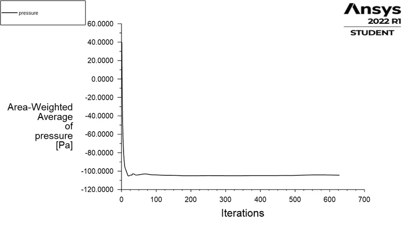
Avg.Static Pressure = 104.352 pa

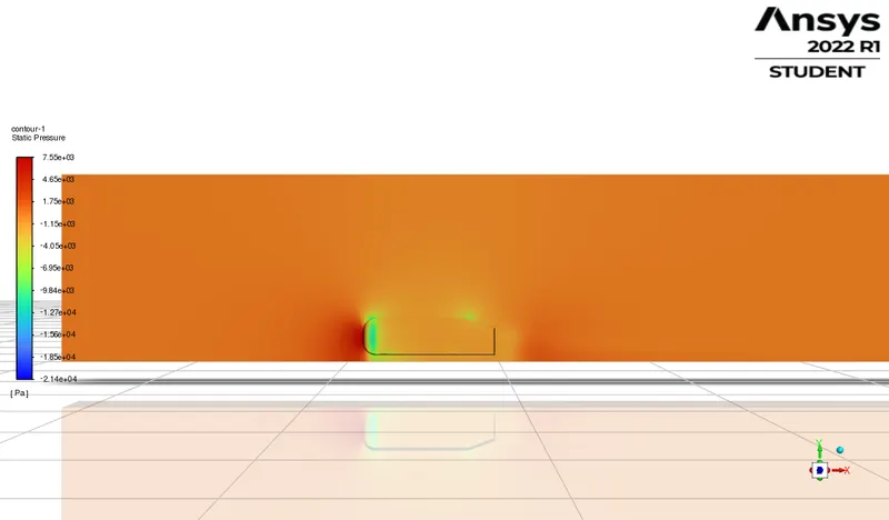
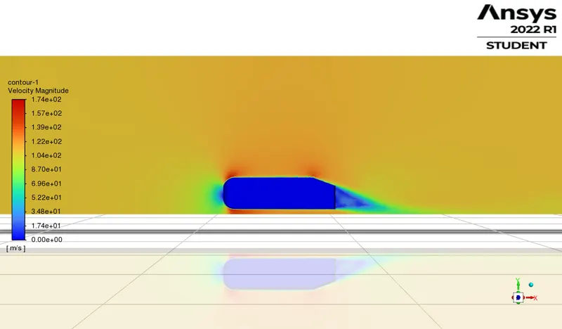
Velocity -

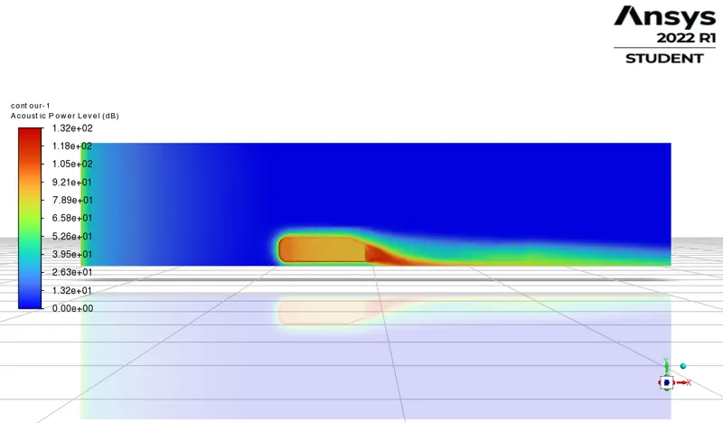
Acoustic Power Level -

Conclusion :

From the above contours and plots we can confirm that the solution converges and the velocity and pressure field is visuvalised. We use the brodband model as turning it ON will enable us to alos solve for the turbulant acoustic phenomeon and do required observation like,the above contour where we can see the noice power and the noice source.