Week 1- Mixing Tee

Aim:

In this part we find the resultant temperature and velocity in a pipe where we mix air at two different temperatures.

Theory and Inputs:

Since the two inlets and an outlet makes the shape of 'T' we call this setup as Mixing tee. We choose air as the working fluid at parallel and perpendicular inlets with temperature 36°C and 19°C respectively. Inlet velocity for Hot air will be 3 m/s.

We simulate the above given conditions for two different lengths of the pipe. And in addition to that the simulation is done for momentum ratio 2 and 4 for both the cases.

Momentum ratio = (Velocity of Cold Inlet) / (Velocity of Hot Inlet)

To begin with we have to first decide for what model of Renylods average Navier Strokes model is best for this simulation, we have to choose between k-epsilon and k-omega model. And then use that model to simulate for different cases.

Therotical formula

Tout=Tmix = `((mhot* Thot ) + (mcold * Tcold))/(mcold+mhot)`

m= `rho *A*V`

Thot = 36°C

Tcold = 19°C

Procedure:

• With the given momentum ratio we have to determine the velocity at cold inlet. Therefore we arrive at two velocities for two ratios.
• We start the new project and import the geomentry in space claim.And specify the volume in contact with our working fluid and seperate it for studying its physics.
• Then we open the Mechanical interaction to generate mesh. And we have to mention the different faces for boundary condition and name them. Then we generate for the default mesh sizeing.
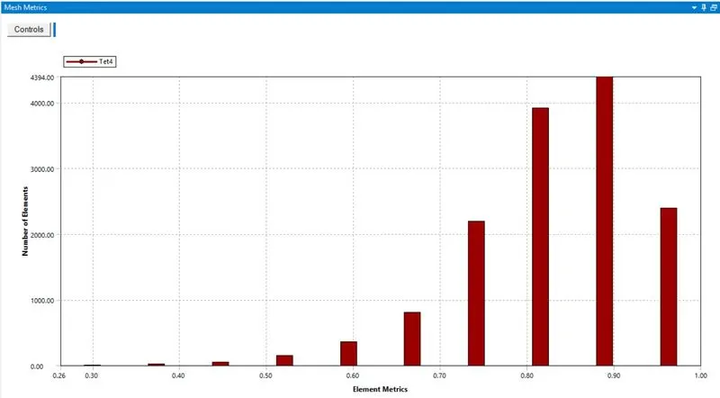
• The quality plot of the generated mesh shows us the no.of mesh vs quality and the bar shouuld be high towards 1 and low bar in the region below 0.5 by this way the most of the cells are of higher quality and so will be the results.

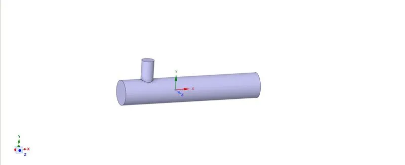
Volume of Interaction with the fluid.

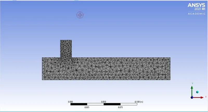
Generated Mesh Cross-Section at 5e-3 m.

• Then we open the fluent interaction where we have to specify various conditions, equations for simulation.First we have to choose the suitable turbulance model. So we chose the viscous model and we choose any of k-epsilon or k-omega SST model. then we have to givet mention the given data for temperature and velocity. We do this once for each model. We then initialise the solution and make sure the solution converges. And iterate the condition till the results converge.
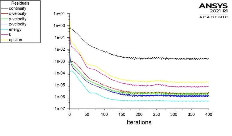
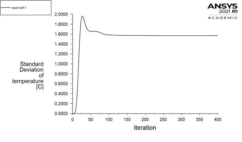
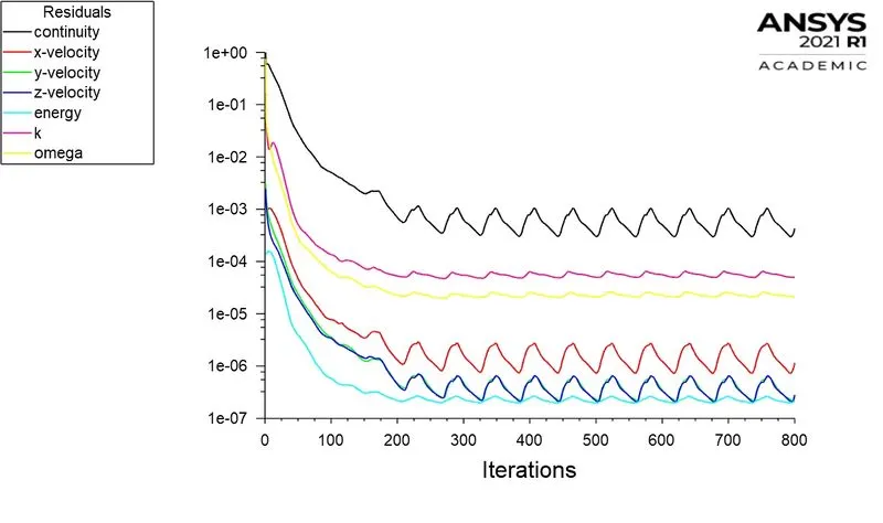
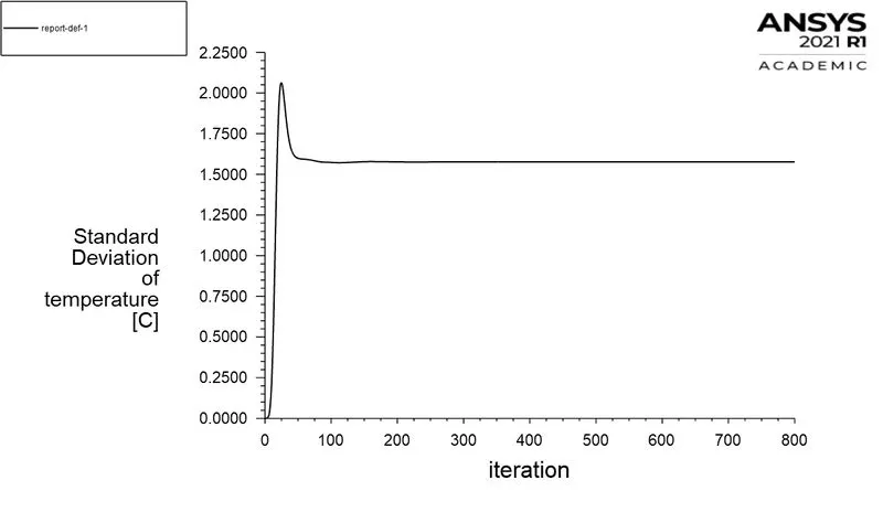
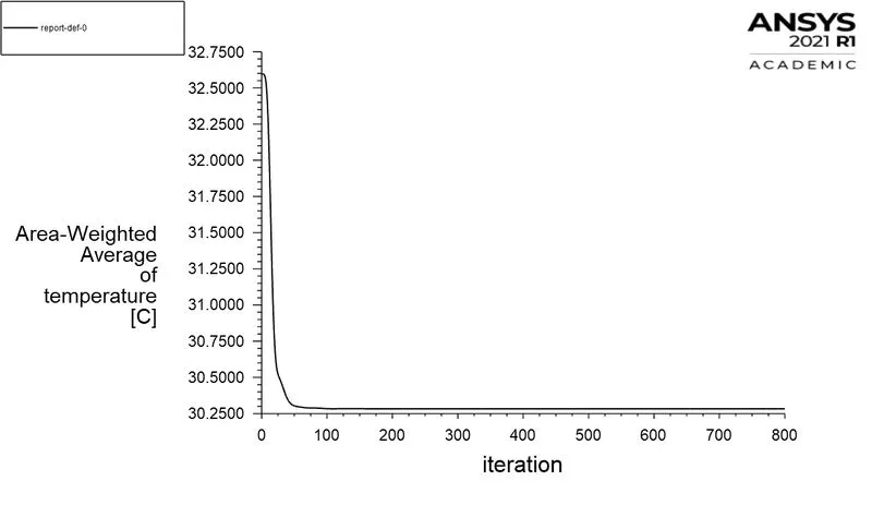
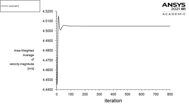
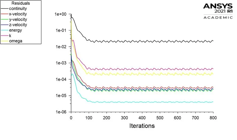
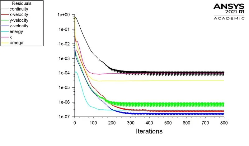
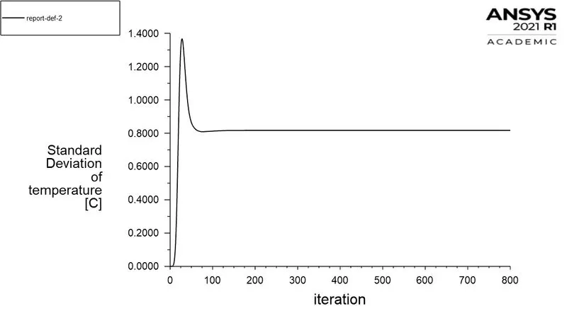
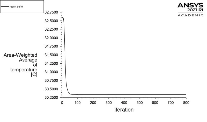
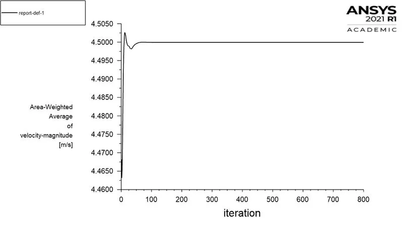
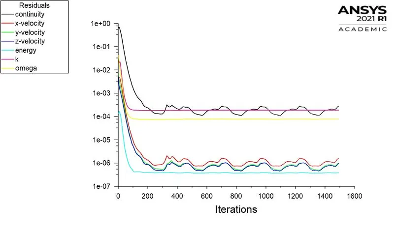
• For the results part we need to obtain the Area weighted average of velocity and temperature in exit and the standard deviation of temperature to check if the results are close to each other at the exit. Along with this we also plot the graph for resuidals of equations that are solved and check for their convergence.

K-Epsilon vs K-omega:

The below plots are thus plotted accordingly for both modles, to determine the suitable model for further simulations. We have taken the resuidal and standard deviation plot for comparision.

K-epsilon

K-omega:

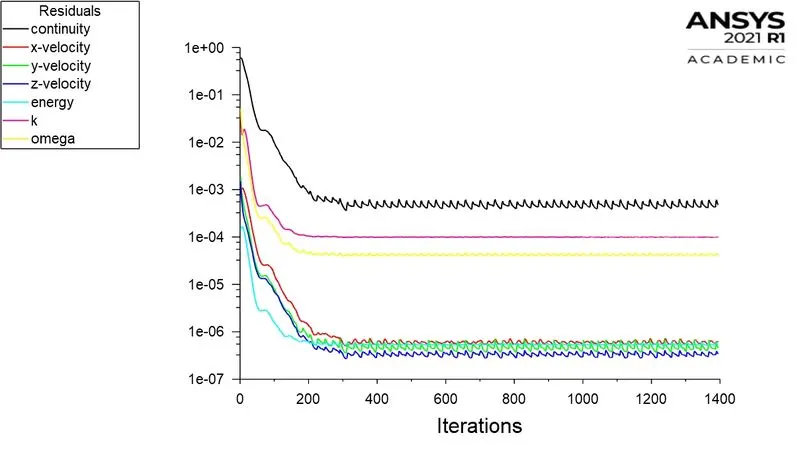
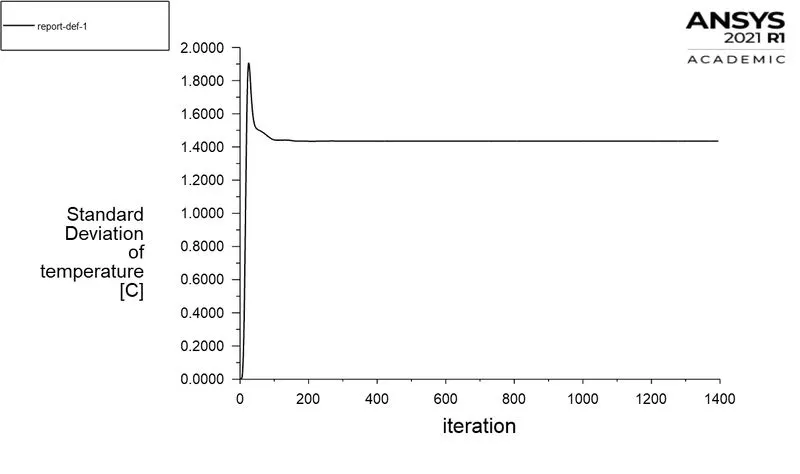
• We do this so that the results obtained are more accurate for this type of simulation. We use hybrid model for solving additionally we also solver for energy equation. from the above resuidal greph for both cases we can observe the solution converges approximately at 200th iteration for k-epsilon model and at aproximately at 450 th iteration for k-omega model.And since the k-`omega`model takes longer time with more accurate results we choose it for further simulations in this case.
• Further on we use this same initial conditions with the k-`omega` model to simulate for Short mixing Tee.

Short Tee: 0.1924 m

• Before we start for the actual simulation we do the 'Mesh Independent study' for the Short Tee with Momentum ratio 2. For this we generate mesh for paticular sizing and obtain its respective outlet temperature.
• We start from geomentry where we choose short-Tee geomentry then we generate mesh for a paticular sizing and then progressively reducing the mesh size.the in fluent after convergence we obtain outlet temperature. This procedure is done for four cases.

S.No	Mesh Size	No.of Elements	No.of Nodes	Avg.Temperature (°C)	Avg.Velocity(m/s)
1	1.021e-2	12583	2797	30.25775	4.4969
2	5e-3	14247	3142	30.283379	4.5047
3	3e-3	39817	8350	30.323525	4.4944
4	1e-3	105858	21330	30.413681	4.5063

• As we could see that at fourt iteration the change in drastic the mesh size is not reduced further. the average temperature is more accurate as we decrease the mesh size. What we need is , the temperature to be accurate and the simulation to be nominal and not not long. So we simulate further for the mesh condition in second case.

Inlet Conditions:

• Velocity hot = 6 m/s
• Velocity cold = 3 m/s
• Temperature hot = 36 °C
• Temperature cold = 19 °C

@ Momentum Ratio =2 ,

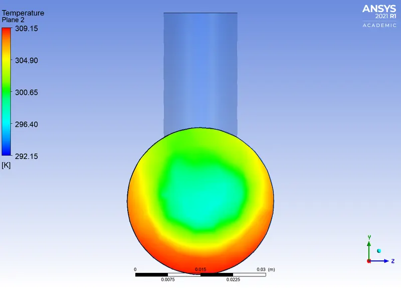
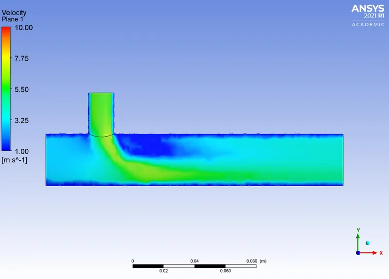
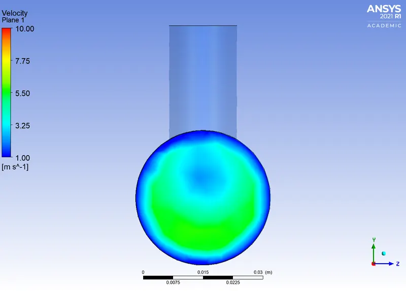
Contour:

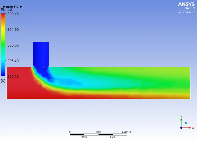
• For plotting the Temperature and Velocity contour we open CFD post.
• We then insert the plane in paticular plane we want the result to be and then change the color to variables of temperature and velocity.

Temperature along the length

Temperature across the length

Velocity along the length

Velocity across the length

Result:

Avgerage Temperature = 30.283265 °C

Theoratical Temperature (Tmix)= 30.32 °C

Average Velocity = 4.5047719 m/s

Standard Deviation = 1.5761 °C

@ Momentum Ratio =4,

Inlet Conditions:

• Velocity hot = 12 m/s
• Velocity cold = 3 m/s
• Temperature hot = 36 °C
• Temperature cold = 19 °C

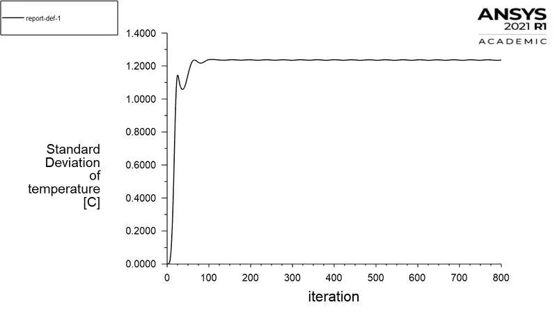
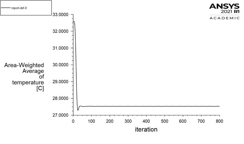
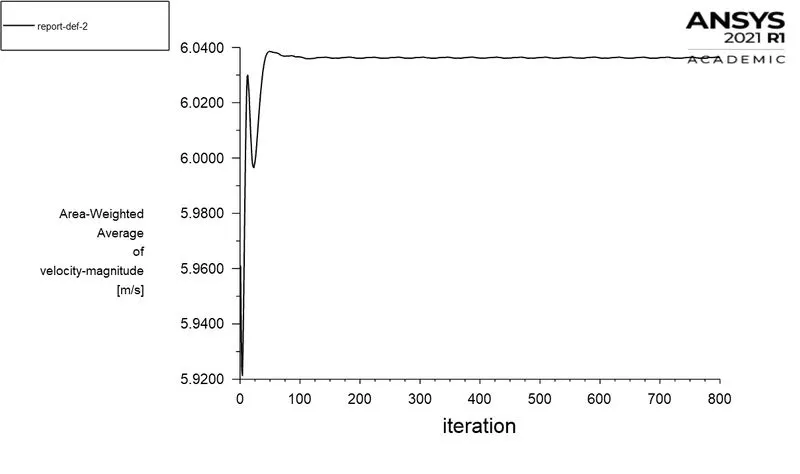
Contour:

Temperature along the length

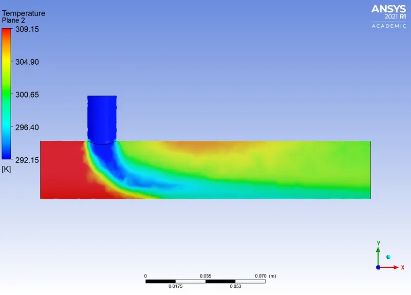
Temperature across the length

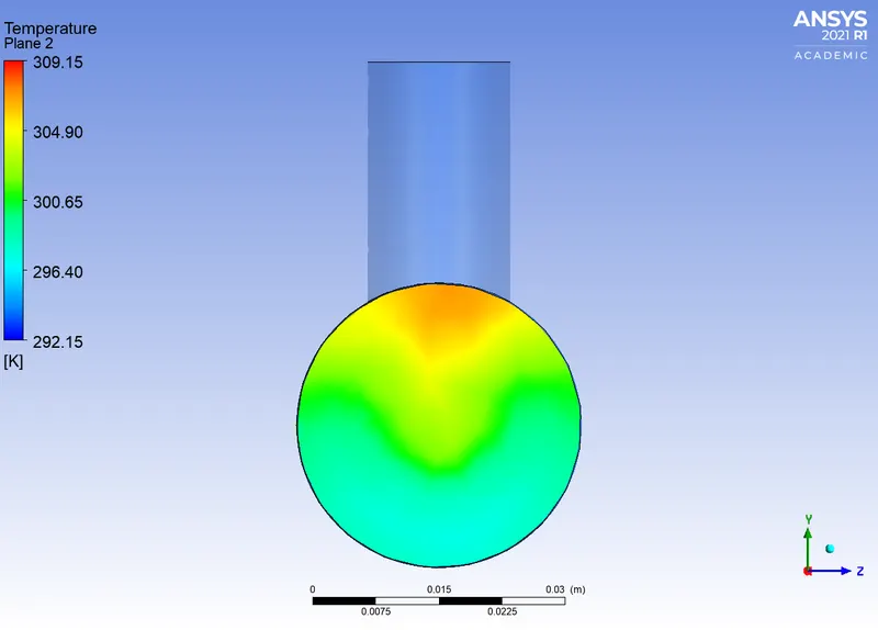
Velocity along the length

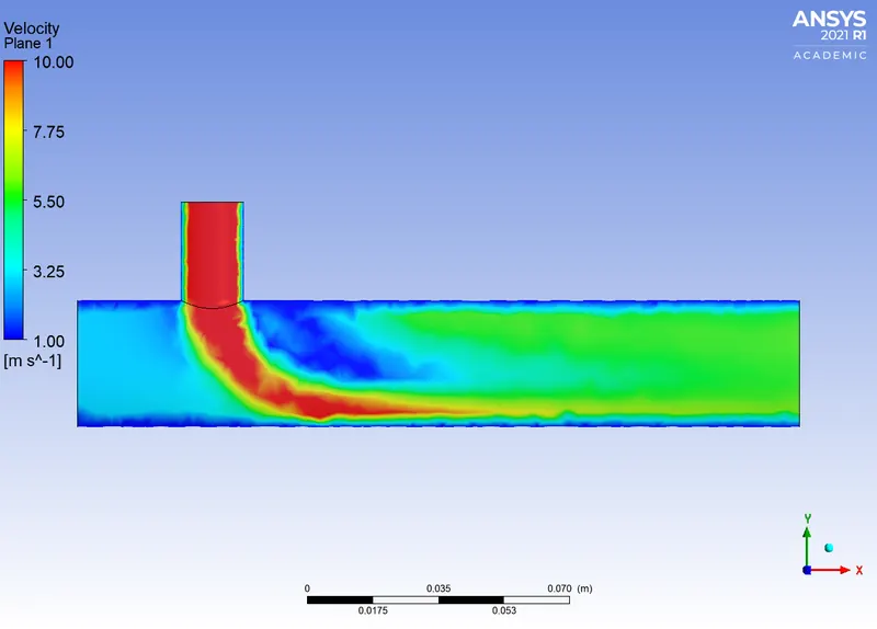
Velocity across the length

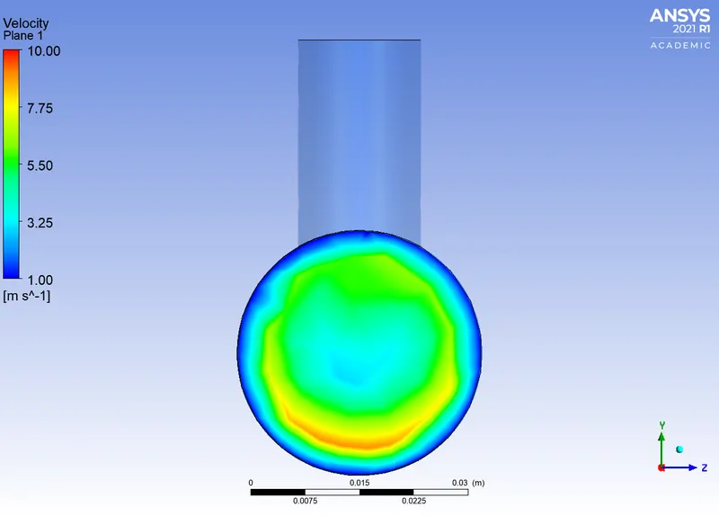
Result:

Avgerage Temperature = 27.530028 °C

Theoratical Temperature (Tmix)= 28.487 °C

Average Velocity = 6.0363181 m/s

Standard Deviation = 1.2362891 °C

Long Tee: 0.2683 m

Inlet Conditions:

• Velocity hot = 6 m/s
• Velocity cold = 3 m/s
• Temperature hot = 36 °C
• Temperature cold = 19 °C

@ Momentum Ratio= 2

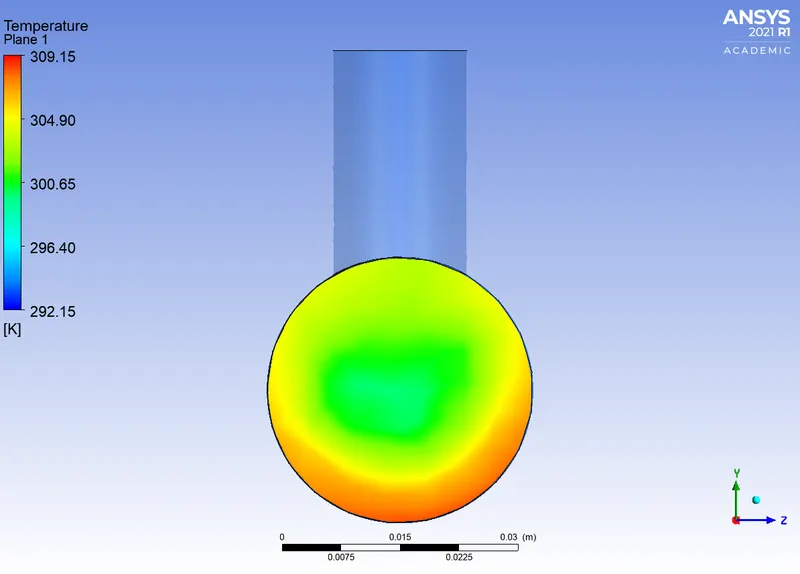
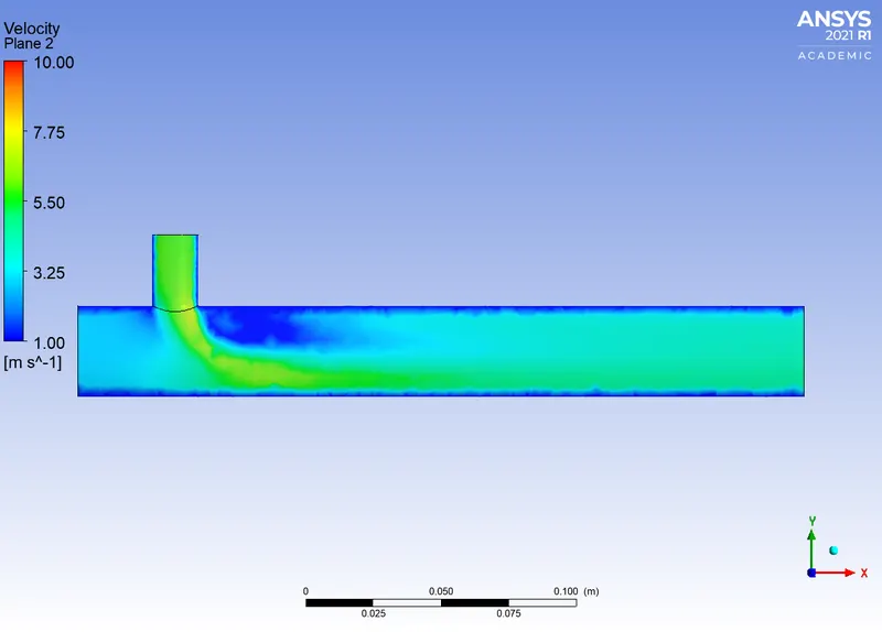
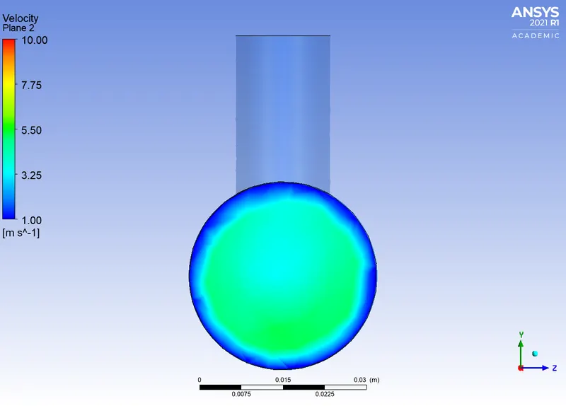
Contour:

Temperature along the length

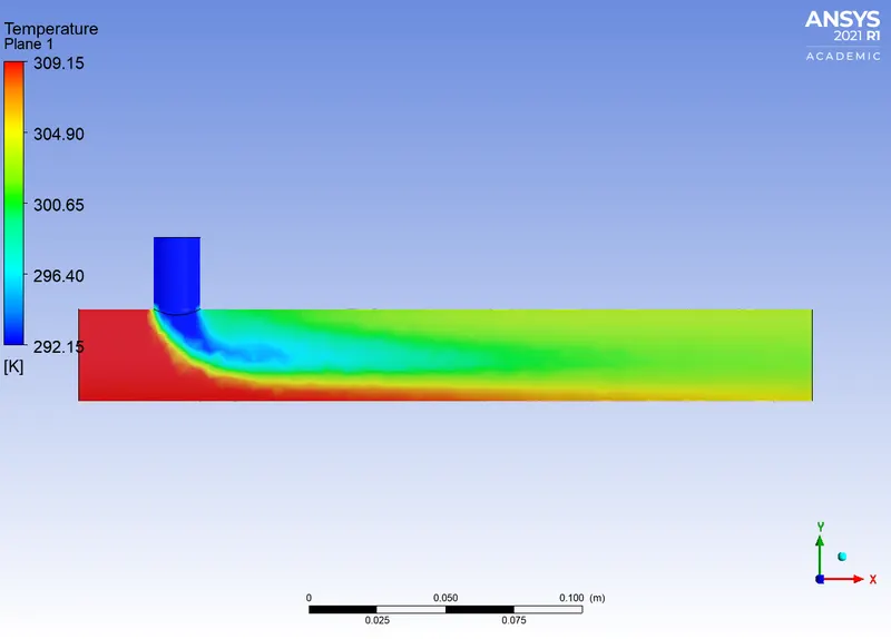
Temperature across the length

Velocity along the length

Velocity across the length

Result:

Avgerage Temperature = 30.339181 °C

Theoratical Temperature (Tmix)= 30.32 °C

Average Velocity = 4.499 m/s

Standard Deviation = 0.81688 °C

@ Momentum Ratio=4,

Inlet Conditions:

• Velocity hot = 12 m/s
• Velocity cold = 3 m/s
• Temperature hot = 36 °C
• Temperature cold = 19 °C

Contour:

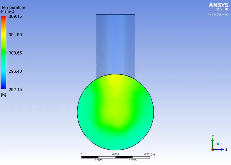
Temperature along the length

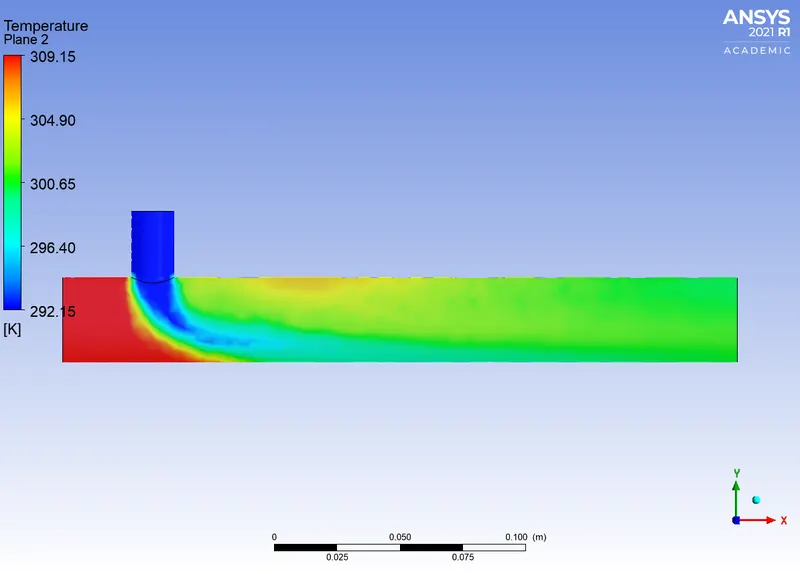
Temperature across the length

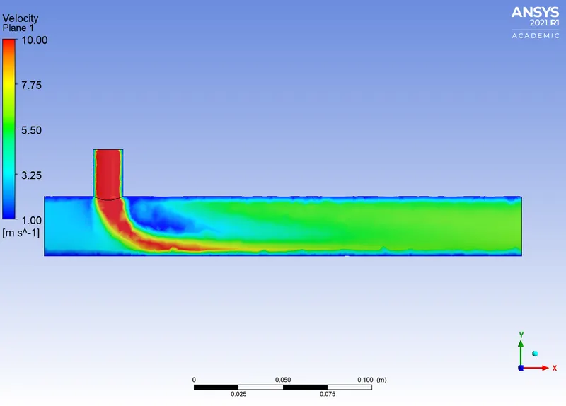
Velocity along the length

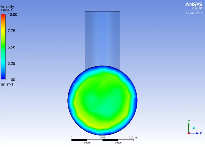
Velocity across the length

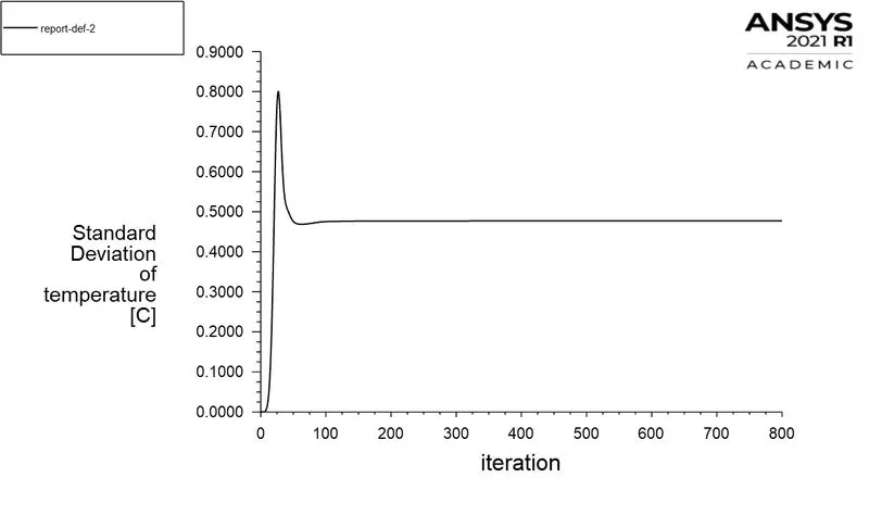
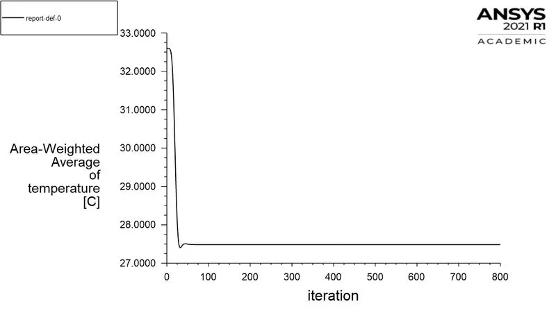
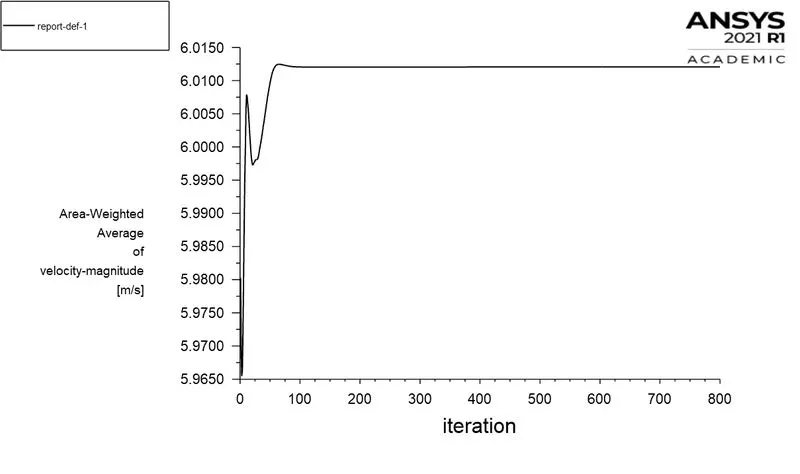
Result:

Avgerage Temperature = 27.481431 °C

Theoratical Temperature (Tmix)= 27.487 °C

Average Velocity = 6.01205 m/s

Standard Deviation = 0.4770134 °C

Conclusions:

	Ratio	No.of Elements	Avg.Temperature (°C)	No.of Iterations	Inlet velocity cold (m/s)	Temperature Cold (°C)
Shot-Tee	2	14247	30.2832	200	6	19
	4	14247	27.5300	220	12	19
Long-Tee	2	17787	30.3391	325	6	19
	4	17787	27.4814	350	12	19

• Therefore from these results we can conclude that the average outlet temperature depends on the velocity and the temperature of the inlet not the length of the pipe.
• Since the velocity Inlet cold is propotional to Momentum Equation the outlet temperature is propotional to it.