Week 8 - Simulation of a backward facing step in OpenFOAM

In this following problem we are dealing with an Incompressible Laminar-Viscous flow inside a domine.

Incompressible flow: A flow in which density remains constant throughout.

Laminar : A flow in which the fluid particals travels smoothly over each other (ie.Re<2300). And there is less friction between the flow particels.

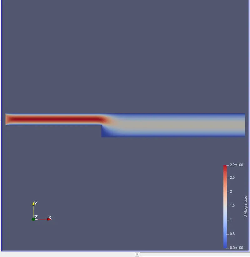
Viscous Fluid: The fluid which has higher viscosity( the measure of internal resistance between adjusent layers of a fluid). It depends on the fluid density, temperature ,pressure etc..The fluid flows in layers, the layer which is close to a solid wall have zero velocity, and have high viscosity this is called no slip condition. The velocith along the axis of the domain will me maxium and hence called Invicid region.

Procedure :

1. First we open the transcript and enter the command to Open Foam.
2. The we change the directory to tutorial.
3. Since it is a Incompressible flow we open the incompressible file. And since we deal with laminar viscous flow we select 'icofoam' solver. icofoam solves for Incompressible Laminar flows.
4. And Inside we choose cavity folder as it holds the option to open and edit mesh files and constants for bouandary conditions.
5. Then we copy the cavity folder inside it to $FOAM_RUN folder, where we can test run the solver.
6. We then change directory to foam run. where we open the cavity folder inside the copied file.
7. In that we choose systems file where we can find mesh file and controlDict to change mesh and runtime respectively.
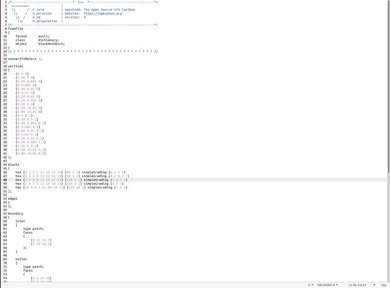
8. We open mesh file and edit the vertices,inlet ,outlet,and fixed walls alond x,y,and z directions. We define five blocks in the mesh each blocks is made up of eight vertices so we use 'hex(...)' command to define then we specify how many cells should it have in each axis(ie (200,20,1)) then we mention the grading factor along each axis.
9. The boundaries are generated by mentioning the faces that corresponds to the inlet and outlet and by mentioning the faces corresponding to the fixed wall. For each faces to be specified we use the previously defined vertices ,and four vertices makes one face.
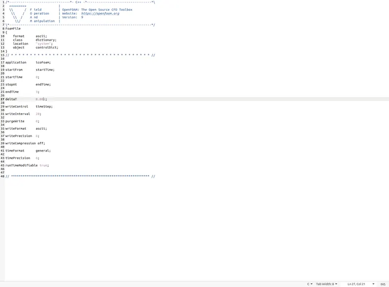
10. Then we open the controlDict file using 'gedit controlDict' an dthe change the end time to 3 sec and time step dt to 1e-2.
11. Then we use 'cd ../' command to go previous and open initial case '0' folder where we find constants pressure p and velocity U.
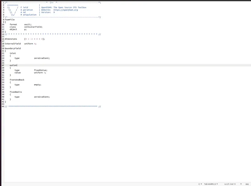
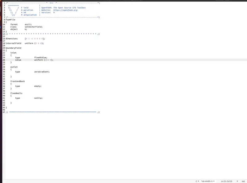
12. We change the inlet velocity to 2 m/s along x axis and pressure to zerogradient.
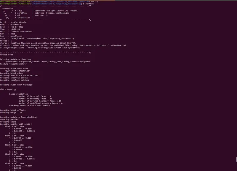
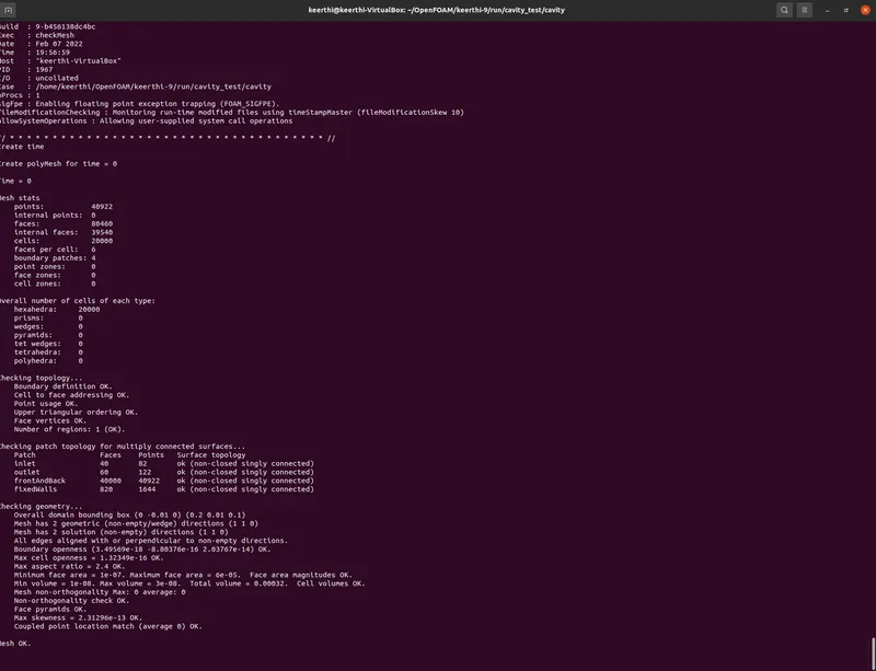
13. Finally we revet back to cavity folder copied and initiate the mesh file using 'blockMesh' command and generate mesh and chech the mesh file using 'checkMesh' command.
14. Thene we use 'icofoam' command to run the simulation .
15. Thereafter we open the paraview to visuvalise the results.

Generating Mesh:

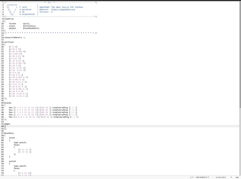
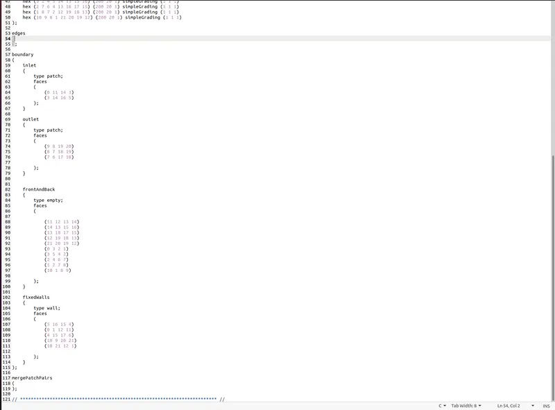
Changing the end time and time step:

Sepcifing Inlet Pressure:

Specifing Inlet Velocity:

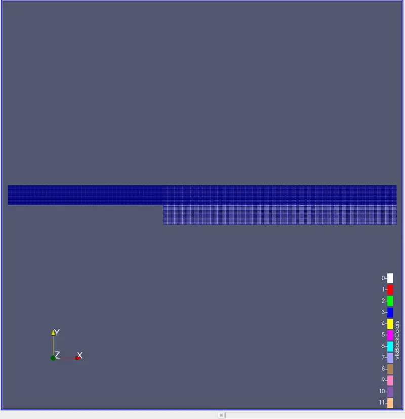
Generated Mesh:

Checking if the mesh is generated successfully without Error.

Generating mesh with proper distribution of cells and with grading factor 0.2 for finer cells along the walls.

Results:

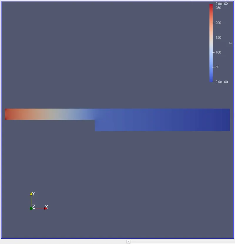
The following outputs are without grading factor

Pressure Contour:

Velocity Contour:

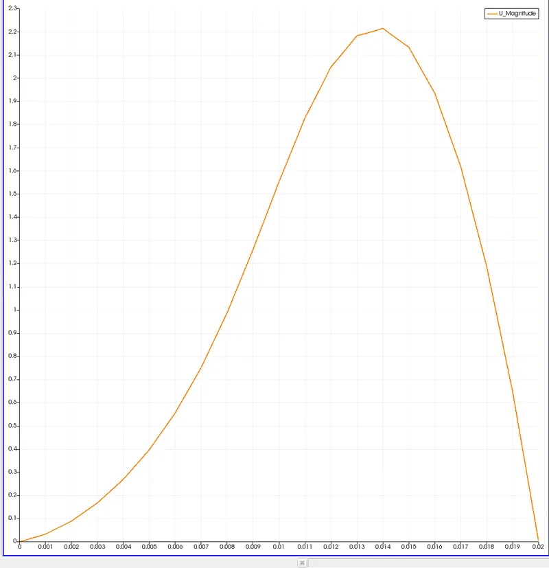
Velocity Plot:

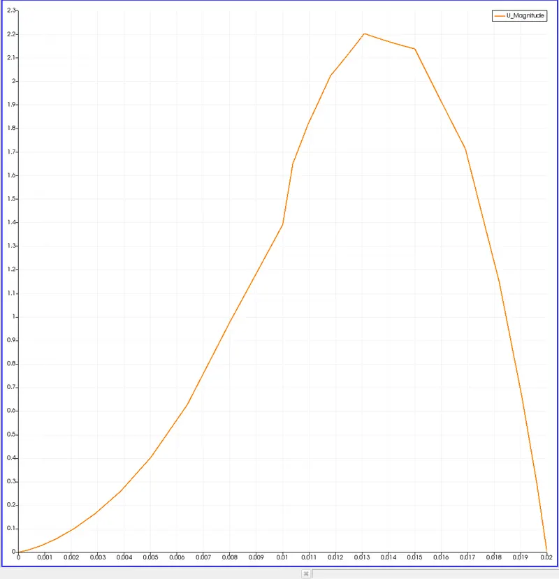
This represents the change in velocity along y-axis at point 0.085 ,just after step wall.

With grading factor 0.2:

Mesh:

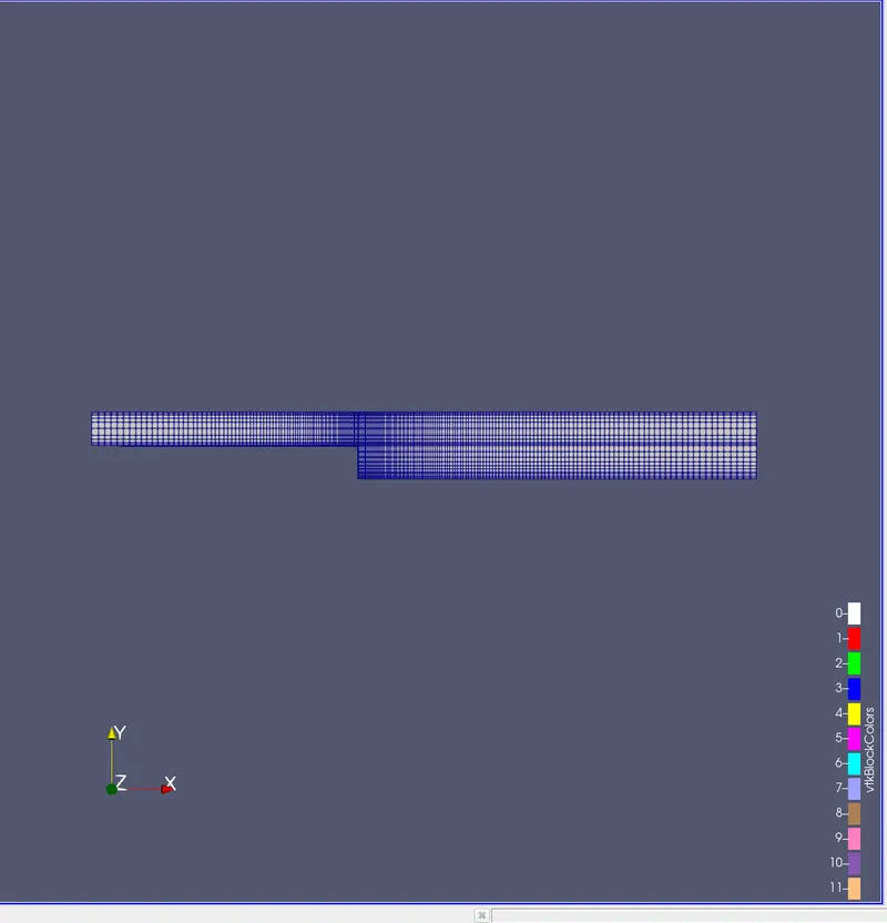
As we can see the cells are finer along the walls.

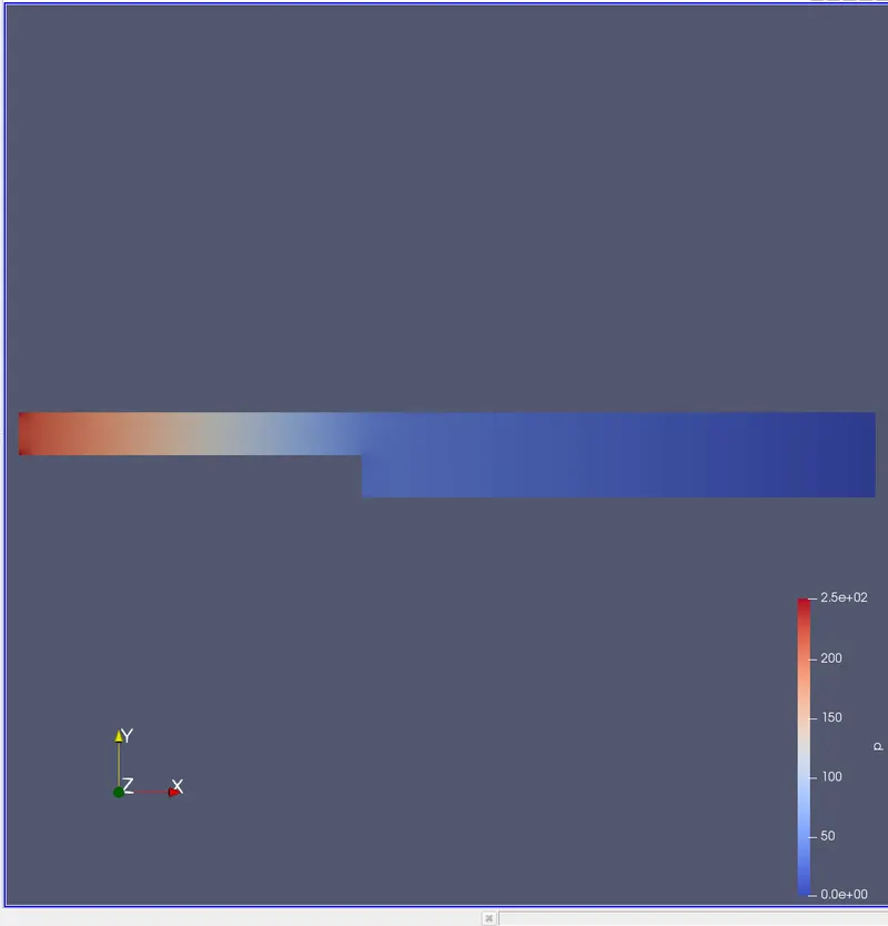
Pressure Contour:

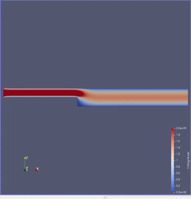
Velocity Contour:

Velocity Plot:

Conclusion:

From observing the line graph we can say that the graph looks smoother for non grading and it is not when we add the grading factor. This can mislead somebody by choosing to go with non graded mesh. Since we added grading factor to have fine cells along the walls and at the step , our intention is to get more accurate results by doing this. And for this reason we get the graph not as smooth as other. We could see the change in velocity clearly from both results and with the use of grading factor we are able to produce near perfect results at a point we desire.

The grading factor helps us to save simulation time by not going for finer mesh alltogeather requires more space ,but to have it at places we wish want to study for. And we can also predict the point along y-axis at which the velocity is maximum more accuratly nearly at 0.013 by using grading factor than at 0.014.