Week 3 - Pitot tube

Aim:

To simulate for the given pitot tube model and obtain necessary results.

Objective:

To calculate the static and total pressure for the given velocity and gauge pressure. And compare the therotical and anylitical results and calculate the error.

Introduction:

Pitot Tube:

A pitot tube measures fluid velocity. It is widely used to determine the airspeed of aircraft the water speed of boats; and the flow velocity of liquids, air, and gases in industry.The basic pitot tube consists of a tube pointing directly into the fluid flow. As this tube contains fluid, a pressure can be measured; the moving fluid is brought to rest as there is no outlet to allow flow to continue. This pressure is the stagnation pressure of the fluid, also known as the total pressure or the pitot pressure. There are three types of pitot tubes Simple, Static ,and Pitot static tubes. they are used to measure Total pressure,Static Pressure, Total and Static Presssure respectivly.

In this model we use Pitot static tube where the center opening is used to calculate the Total pressure and the other openings on the sides is used to calculate the Static pressure.

The relation between static and total presssure is ,

Total Pressure = Static Pressure + Dynamic Pressure

Which can also be written

Solving that for flow velocity gives

where

• is the Flow Velocity
• is the stagnation or total pressure;
• is the Static Pressure
• is the fluid density.

The above relations hold only when the aircraft is flying at low speeds and so that the air in front is incompressible.

Procedure:

• First we import the mesh file of the model directly instead of opening it in geomentry. For this we don't require the fluent solver under "Solver System" but the fluent standalone system under "Component System". Where it only contains setup and solution part.
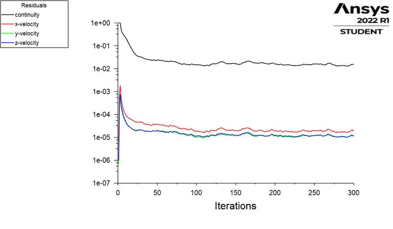
• For setting up the physics consider it as a presssure based stady state solution. Under viscous model we choos the laminar model for solving.
• The reason to choose this model is because the flow is simple and there is no resisrtance to the flow along its path. Further since in pitot tube the pressuredrop will be neglegible and therefore in laminar flows the pressure drop per unit length is lesser than Turbulant flow.
• Next we define the boundary conditions at inlet and outlet. The velocity and corresponding gauge pressure are given as,

Velocity(m/s)	Gauge Pressure (Pa)
240	-2817
100	33287
62	65780

• We measure the Total and Static pressure from the defined regions. And plot the graph.
• Under Operating conditions we make the gauge pressure as Zero else it would add to the total gauge pressure ,as we already defined it in Inlet.
• Finally we initialize the solution from Inlet. And run the case for 300 iterations.

Result:

Case1 -

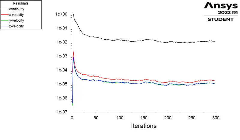
Residual

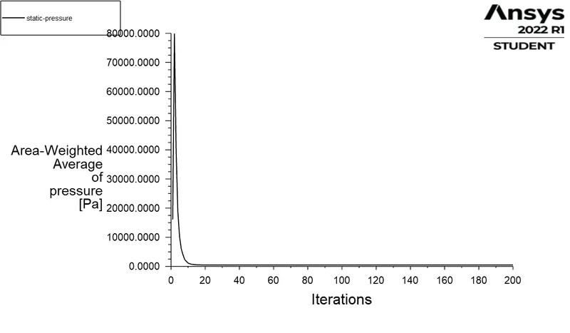
Static Pressure

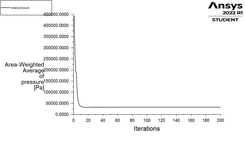
Total Pressure

Contour

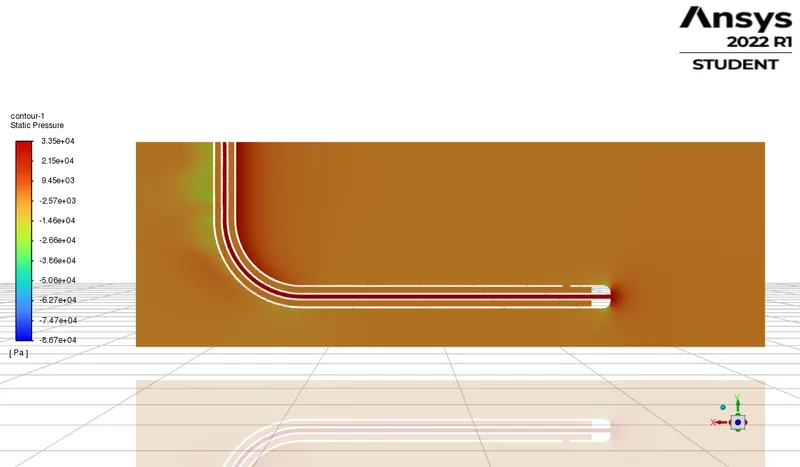
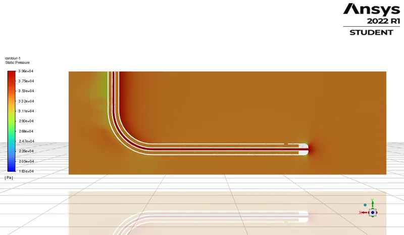
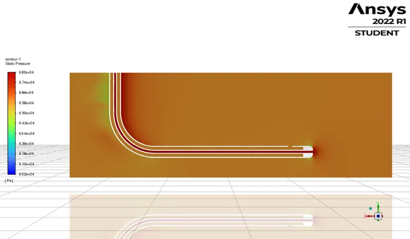
The middle region of higher pressure is the Total pressure region and is where the pressure is calculated. The lesser pressure region sourrounding it is Static pressure region.

Case 2 -

Resuidal

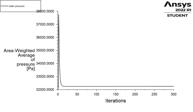
Static Pressure :

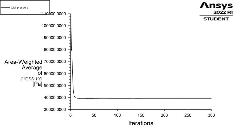
Total Pressure :

Contour :

Case 3 -

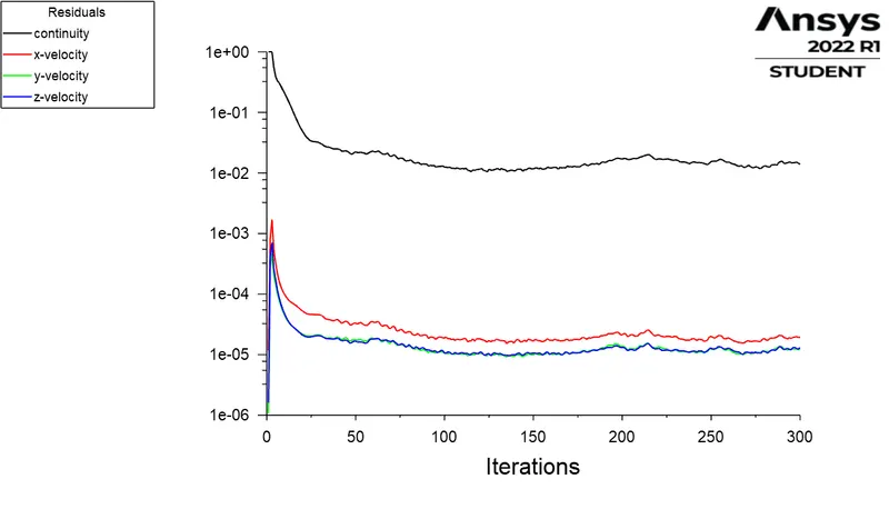
Resuidal

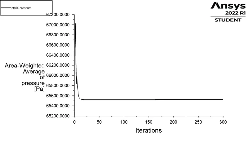
Static Pressure :

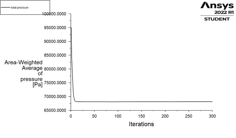
Total Pressure

Contour

Conclusion :

	Theoratical Velocity (m/s)	Gauge Pressure (pa)	Static Pressure (pa)	Total Pressure (pa)	Analytical Velocity (m/s)	Error Percentage (%)
Case 1	240	-2817	467.5094	32639.811	229.167	4.513
Case 2	100	33287	32250.857	35450.871	105.421	5.421
Case 3	62	65780	65523.989	68148.858	65.476	5.606

The Theoritical and actual velocity error is only around 5 % , which is accectable in induatrial standards. Therefore the simulation is carried sucessfully.