Week 6 - CHT Analysis on a Graphics card

Aim:

To Perform a steady state conjugate heat transfer model on a GPU. And find maximum teperature and heat transfer coefficient of the processor.

Objective:

1. To run the simulation for three velocities 1 m/s,2.5 m/s ,and 5m/s and discuss the results.
2. To find the maximum temperature and Heat Transfer Coefficient attained by the processor.
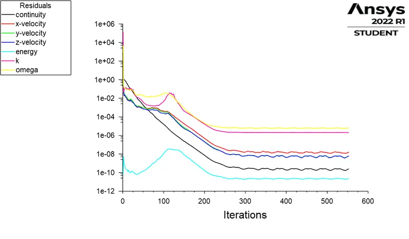
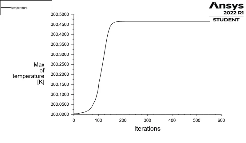
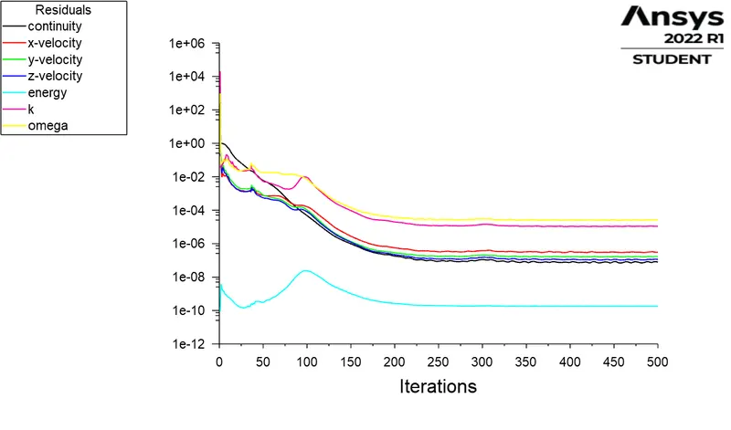
3. To prove the Results are converged.
4. To Identify the potential hotspots.

Introduction:

GPU:

A Graphics Processing Unit is an important component in every high performance computer where the usage of graphics rendering is high apart from this other application such as gaming and AI also requires high performance. The GPU contains a Processor which acts as a CPU , a circuit board , a heat sink(fins) and other electronic components. Over the years the size and performance of GPU steadily increases as a result the processor tends to do multiple processing at a time, this leads to over heating of the processor and decreases the processors performance and workflow of the users. So just like any other heat exchangers the GPU also have fins and an fan to improve Convection.

CHT:

Conjugate Heat Transfer is a type of analysis that specifically studies the heat transfer between solid and fluid domain. This helps us in identifing and visuvalize the heat transfer and its associated properties such as rate of heat transfer, and with these results we could maintain the entire system temperature at an optimum level by introducing heat sinks and blowers at a specific location for effective heat transfer. Further these also helps to reduce cost by choosing appropriate materials for the heat sink and the circuit boards. It is specifically mentioned as conjucate, because the transfer of heat is a combination of both convection and conduction process. In industrial purpous computer chip, mechanical parts,turbines and other components needs to be designed robust for effective use under extreme conditions this is the reason why the combination of both process is considered, as in both forced and normal convection fluid always surrounds the solid body.The convection can be forced or natural convection. The CHT approach has an advantage over Finite Element thermal analysis in that wall heat transfer coefficients and their local variations on surfaces are directly calculated within the model rather than based on simplified empirical calculations. The CHT approach therefore has benefits for those applications where heat transfer is either non-uniform or difficult to calculate empirically.

Procedure:

Geomentry:

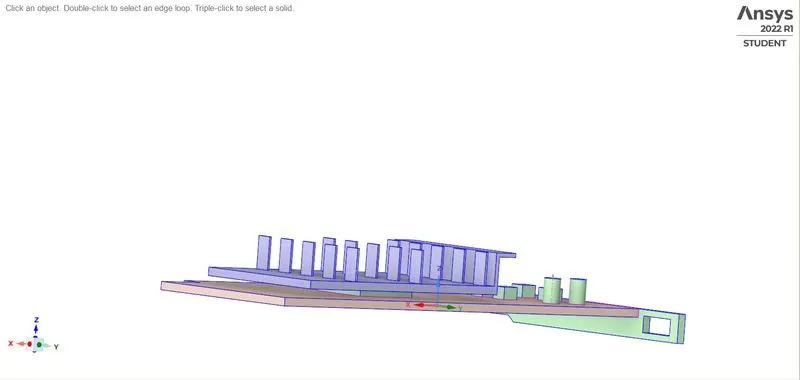
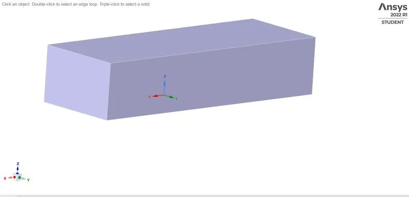
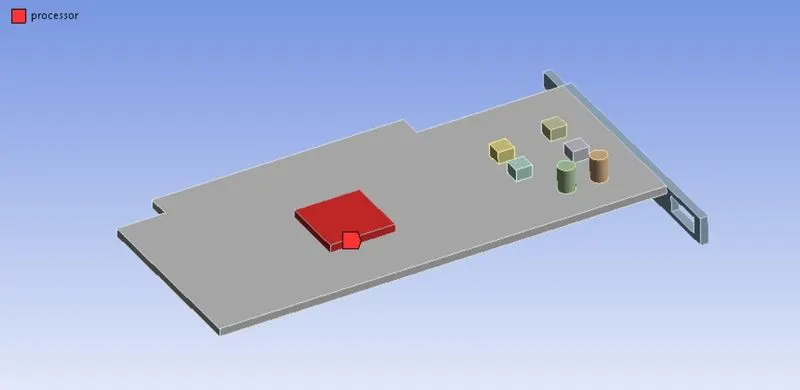
We open space claim and the developed setup is made into an enclosure. Since the entire setup is surrounded by air medium we use this enclosure to create the air medium around the model. Then we prepare the model by sharing the interface region between each model inside the setup. Then we check if the share option is enabled for the entire setup. The processor setup used measures 8mm*8mm*1 mm.

Mesh:

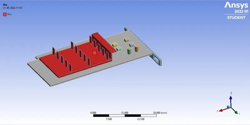
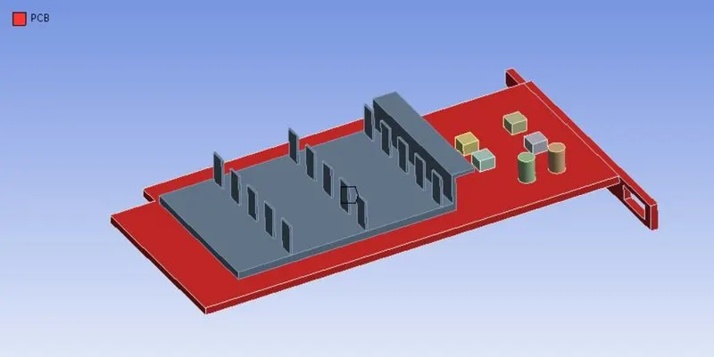
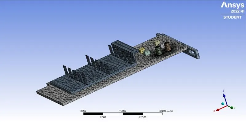
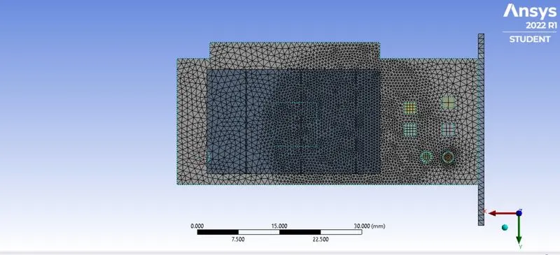
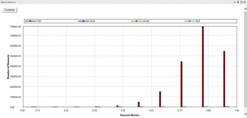
Then we open meshing interface. For this paticular model we take two mesh cases one with default mesh condition and other with refined case . The folowing case is under default mesh condition of 2 mm. Since it is a basic condition the mesh size is constant for the entire setup. For Name selection we have Fins, PCB, Processor and Resistors and capacitors. The entire enclosure is taken as symmentry-wall. The inlet velocity is along the x axis.

Base mesh:

Mesh Size = 2 mm

No.of Elements = 354488

Setup Procedure:

• First we choose the model as k-epsilon, the flow to be steady state flow and the solver as pressure based solver.
• Then we choose energy equation to be solved as we have temperature to be solved for. Then we chosoe the required material for the models.

Fins - Aluminium

Processor - Silicon (User defined)

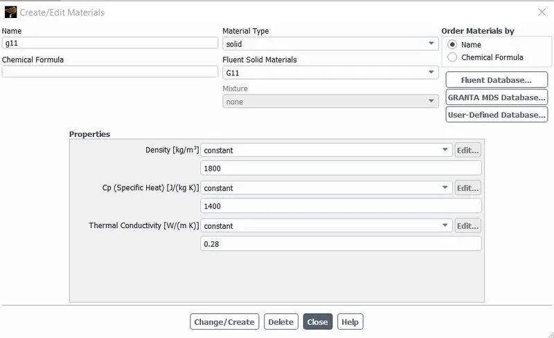
PCB - G11 ( Fiber / User Defined)

Resistor and Capacitor - Copper

Processor

Density - 1800 kg/m^3

Specific Heat - 1400 J/kg.K

Thermal Conductivity - 0.28 W/m.K

PCB

Density - 2330 kg/m^3

Specific Heat - 703.3824 J/kg.K

Thermal Conductivity - 149 W/m.K

This specific G11 is high resistance to solvents, high flexural strength retention at high temperatures. Typically rated to 170 °C.

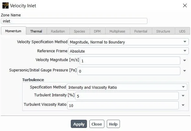
Then we seperate each module inside the system as solid and fluid. And then we asssign each zones its material .Since the processor is the heat source we give Volume Power Density for it. We take the input power consumption of this small processor to be 15W and by dividing this by volume we get 234375W/m^3. For the boundary condition the inlet velocities are 1 m/s , 2.5 m/s and 5m/s therefore we simulated for three cases of velocities. And the temperature at both inlet and outlet is seta as 300 K.

Volume `rho`= 8 *8*1

= 64 `mm^3`

= 64 e-6 `m^3`

Power Consumption = 15 `W`

Volume Power Density = 15/0.000064

= 234357

= 2.34357 e5 `W/(m^3)`

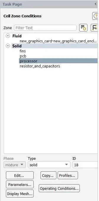
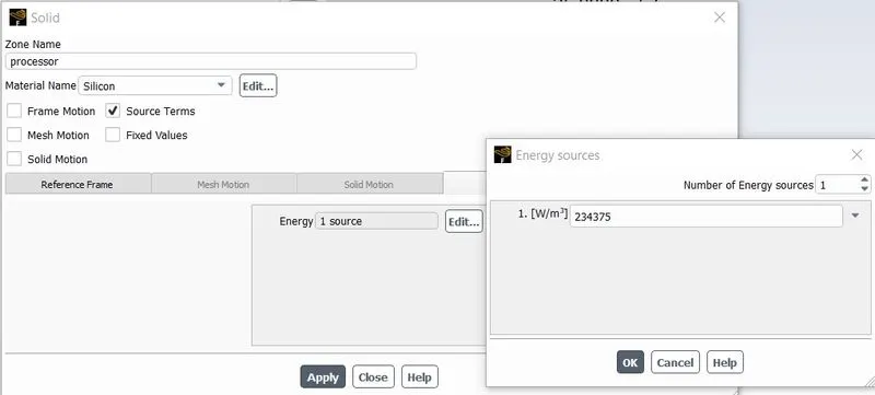
Then we set up the graph to be plotted,

• Maximum temperature at the processor
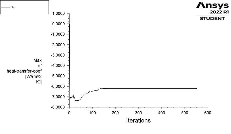
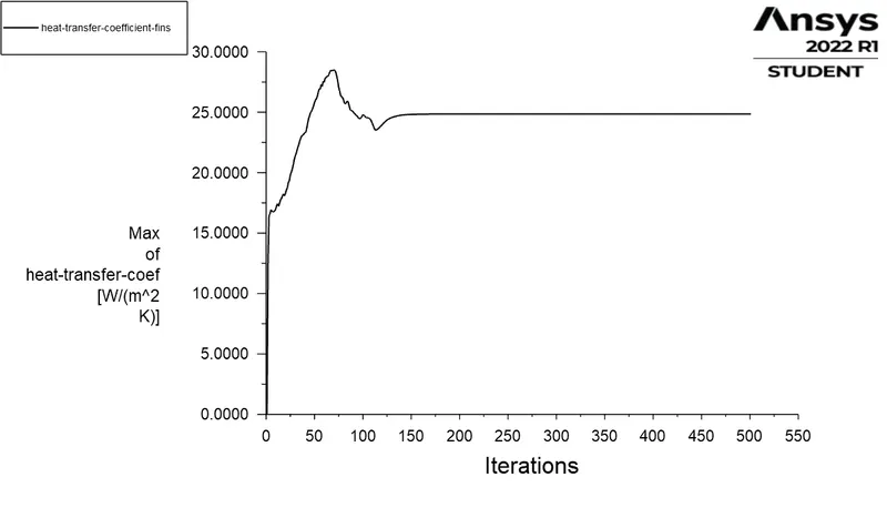
• Heat transfer coefficient of Fin and Processor
• Resuidal

Finally we initialised and ran the simulation for 500 iterations for each cases. And the temperature distribution on fins is visuvalized.

Results and Discussion:

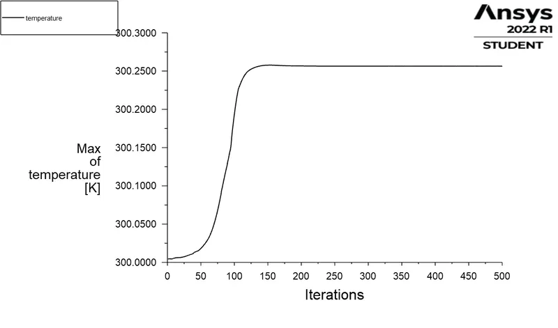
The below mentioned solution is obtained after the solutioun converged. To check for solution convergence , ie the Resuidal plot after 300th iteration have same pattern followed beyond that point so the solutioun is converged. In case of Temperature plot the line is constant after 300 th iteration. This way we can know if the solutioun is converged or not.

Case 1:

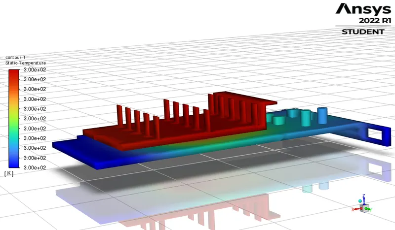
Global Temperature Distribution

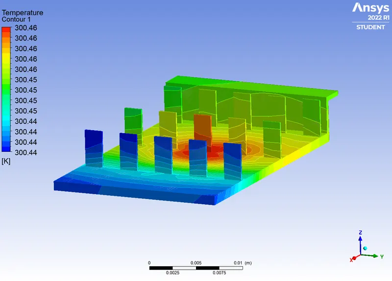
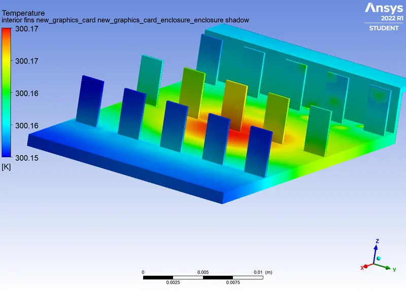
Local Temperature Distribution

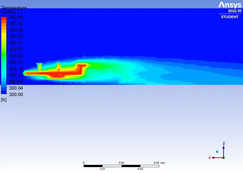
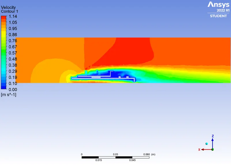
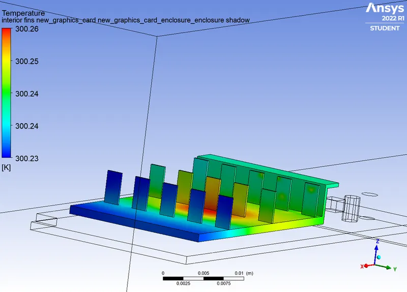
Hotspots At the interface of Processor fin and Processor and PCB

Hotspots - Hotspots are the region where there is only a little cold air flow. This results in less heat transfer at that paticular region.

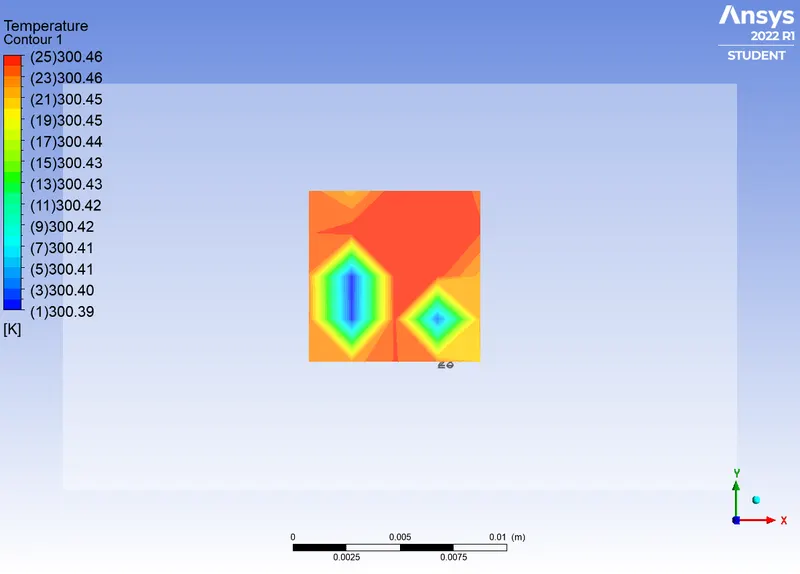
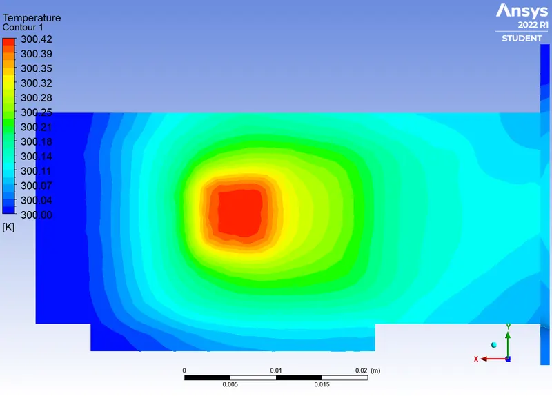
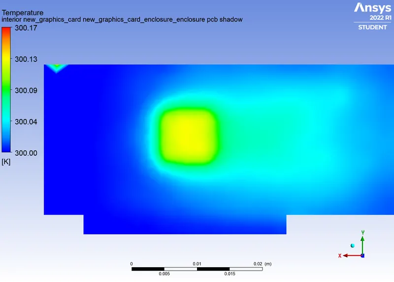
As we can see the hotspots in processor bot interface is obvious as it is the source of heat and more specifically there will be litreally no air passing at its interface as it in contact with solid objects above and below.

Case 2:

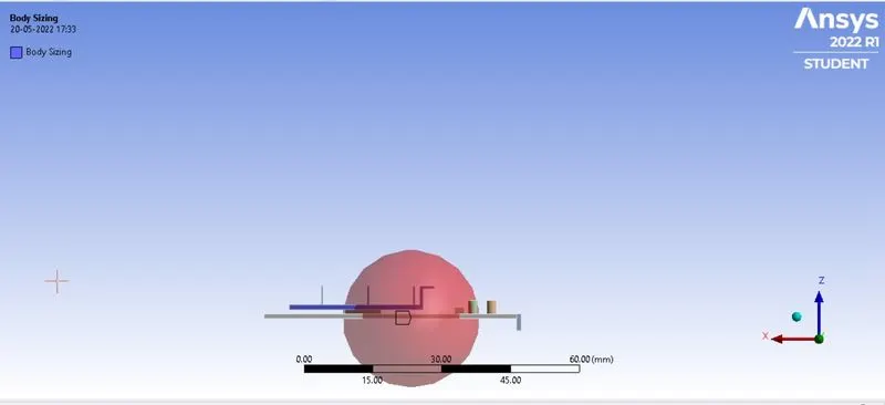
Refinment Mesh

Enclosure - 2mm

Sphere of Influence - 1 mm

No.of Elements - 422147

Inlet Velocity - 2.5 m/s

In this case for refinement of mesh the Sphere of Influence methor is used for meshing only in the area influenced by the sphere. As our focus is to study the processor behaviour and its sourrounding refions this is done to have refinment only in that region.

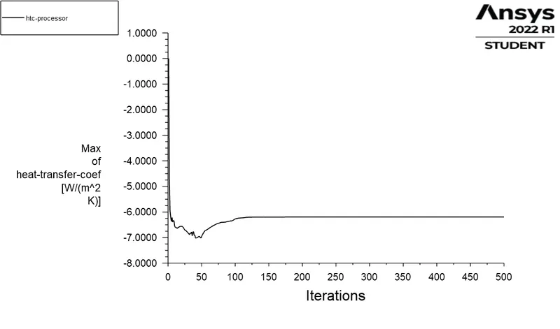
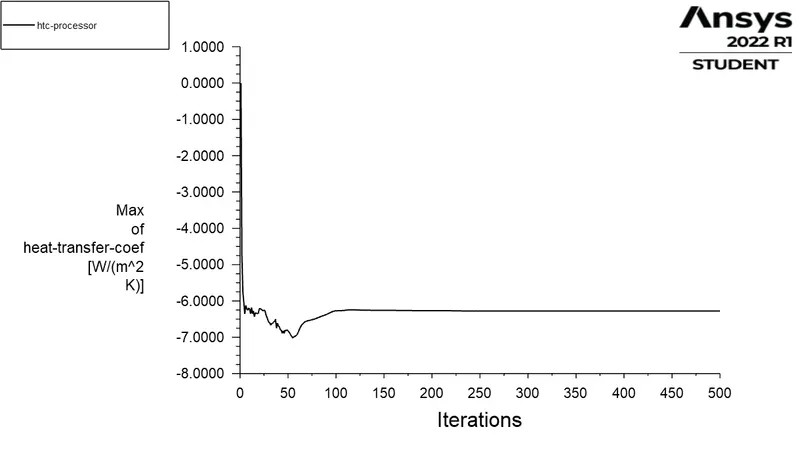
HTC of Processor

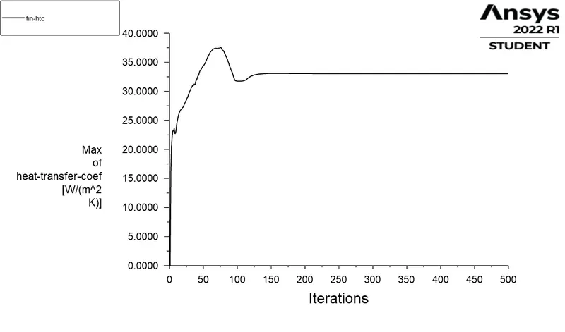
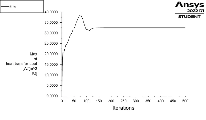
HTC of Fins

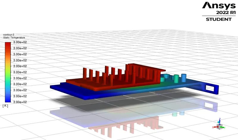
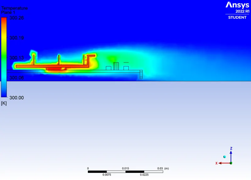
Global Temperature Contour

Hotspots

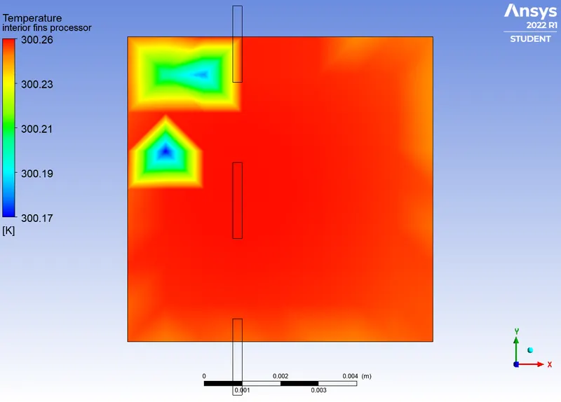
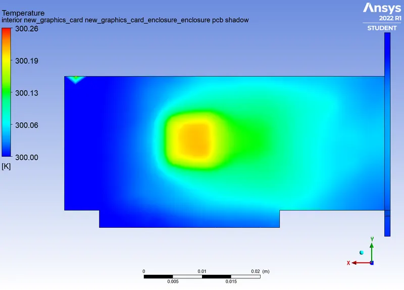
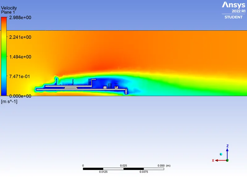
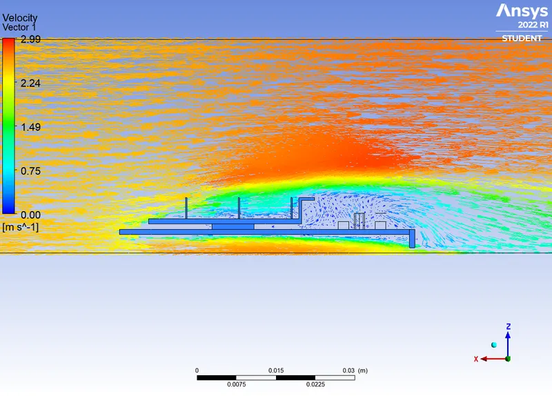
As we can see the temperature contour and the hotspots in this case is more detail and the average temperature around processor is less and above in PCB hotspot. The above representation of velocity vector shows that there is barly any air passing in contact with the processor and the cold air turns hot as it passes over the fins.

Case 3:

Inlet velocity = 5 m/s

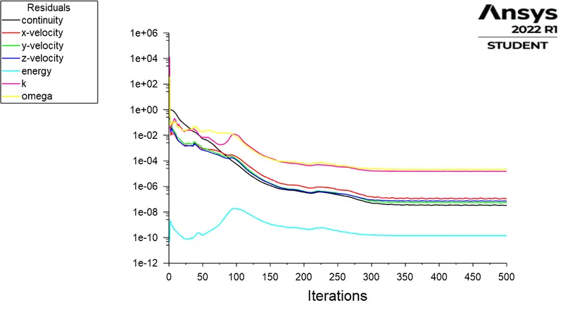
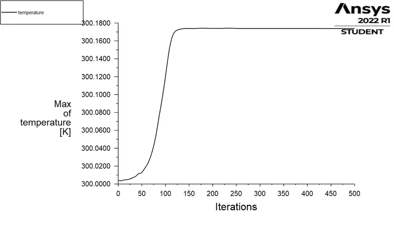
HTC Processor

HTC fins

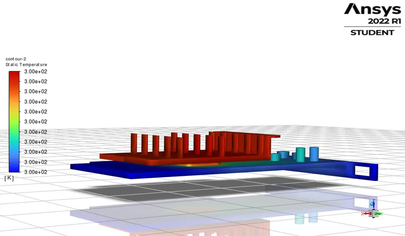
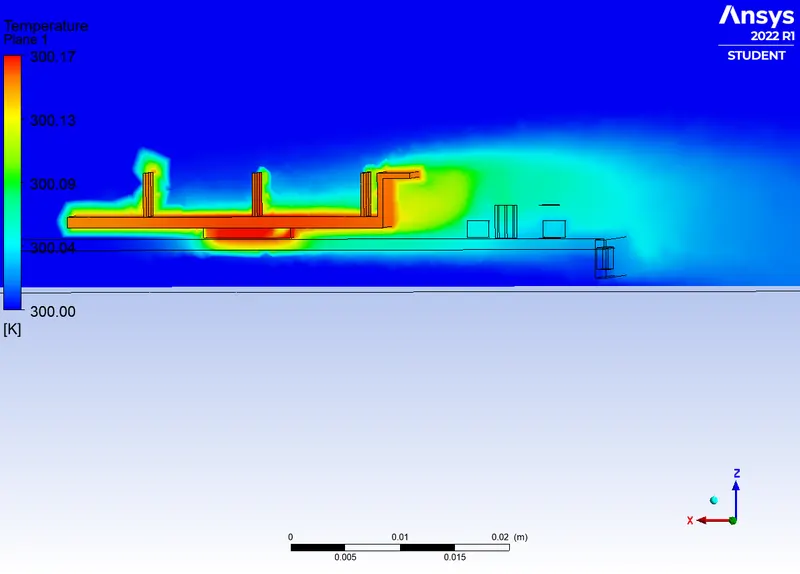
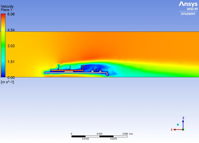
The Region just behind the fin setup and in the region of capacitors and resistors the collection of cold air is because the components does not comes in contact with processor and so they dont conduct or undergo convection.

Hotspots:

Discussion:

S.No	Mesh Condition	Inlet Velocity (m/s)	Max Temperature (Processor) (K)	HTC Processor (W/(m^2 K))	HTC Fins (W/(m^2 K))
1	Basic 2	1	300.4652	-6.2027903	24.85364
2	Enclosure and others 2 Sphere of Influence 1	2.5	300.2565	-6.1948755	33.04577
3	Enclosure and others 2 Sphere of Influence 1	5	300.1738	-6.2773129	32.505625

In this setup we paticularly used sphere of influence because as we refine further as a whole or the fins the elements go past maximum no.of celss allowed . And by this way we can stay within the limit and could only refine the region where majour heat transfer takes place.

As from the above table the Maximum temperature of the processor is decreases as we increase the inlet velocity and mesh refinement. Even with the increase in velocity we saw the temperature of the processor almost remained same but, the heat transfer coefficient of the fins increased this is because the forced convection takes place at much higher rate as we increase the velocity.

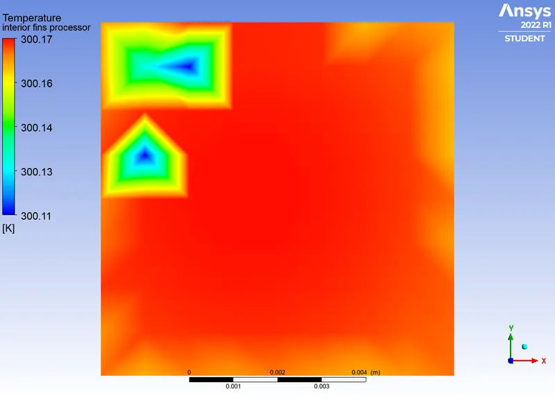
Further When we observe the local temperature for Fins we can see the frontal area of the fins are cooler than the fin section in the middle this is because the heat from the processor conducted through it is very low that,the cold inlet air will cool the frint tin section. The HTC for fins is higher because of higher reynolds number due to higher inlet velocity and since the middle fin section have higher temperature thats the region where majour heat transfer occur and will eventually have higher HTC.

The potential low temperature patches at the far side of the processor is because the fin section above that region effectively conducts heat. And thus simulating an GPU using CHT method is learnt. By this way we can know how many fins to be placed for effective heat transfer and how to decrease temperature at the hotspot regions.