Week 9 - FVM Literature Review

FDM:

In Finite Difference Method discritization is based on differential form of the PDE. The domain is divided into hexagonal cells and the solution will be obtained at each node points. And we finally get a system of equations of variables at nodal points.And once solved we have discrite solution.

FEM:

A Finite Element Method the discritization is based on small elements. The domain is divided in smaller domains or elements.The collection of all these simple shapes constutites the finite-element mesh.Next we take the PDE's and formulate them for each element,and once comined they make up the a large matrix and these matrices can be solved by different solvers.

FVM:

The Finite Volume Method is discritized upon an integral form of PDE.The PDEs are written for a given finite volume or cell. In that way the entire domain is dividen into finite volumes of any arbitery shapes and the governing equation is solved for each volume. The resulting solution comprices of fluxes. The properties are assumed to be at the center of the finite volume .This advantage of eliminating the use of structural grids to a domain , makes FVM preferable over complex structures. Therefore the FVM have a better conservation properties. The fluxes occurs at the surface of the control volume.

Advantages of FVM

• There is no need of converting the Structural grid to a computational domain.
• We can apply FVM to more complex grid points where the adjucent grid points are not in alignment.
• In FDM we have to introduce correction factors to make up for the mis-allignment of grid points, using a method called variable transformation method. Which could get complex and time consuming ass the geomentry of the structure is complex.

Let us assume 2-D heat conduction Equation

`d/dx (alpha * (dT)/(dx)) + S = 0`

`(dT)/dx` - temperature gradient along x-direction

`alpha` - Thermal Diffusivity

`S` - source term

The above mentioned equation is valid not at a point rather to the entire finite volume. Then this equation is is solved by multiplying with as small volume dv in the control volumea and finally when it is integrated over the entire volume and it will be equal to 0, this is called as Integral form of governing equation.

`int((del)/(delx) *((del T)/(delx))) + S ) *dv = 0`

Where,

dv = `A *dx`

S = `Savg`

We use Gauss divergence theorem to conver the volume integral into surface integral.

After integration we arrive at the final Equation with heat flux and source term,

`alpha A[(Te-Tp)/(Delta x)] - alpha A[(Tp-Tw)/(Delta x)] +Savg (dv) = 0`

To solve the above equation we use the following method

1. Gradient Scheme:

We use this scheme to find the temperature between two adjusent finite volumes, for that we use the temperature at the center point of the adjusent cell.And this way of representing the theperature is called as Gradient Scheme.

2. Interpolation Scheme:

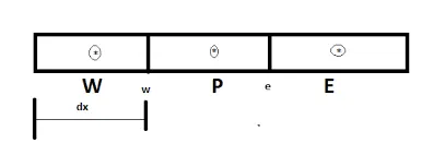
Generally speaking we use Interpolation to find the value at an given point with the points on both sidesof it, whose values are already known to us. In case of FVM we need unknown variables within a control volume, so that we could solve the surface or volume integral at points other than nodes. And to do that we use any of the folowing methods,

1) Upwind Interpolation Scheme:

This scheme solve the solution variable by consediring the direction of the fluid flow. It uses forward and backward difference method.The value at point 'e' is given by , if the flow is from west to east

`fe : Ie approx (u(i)- u(i-1))/ (Delta x)` - Backward Difference`

Flow East to West

`fe : Ie approx (u(i+1)- u(i))/ (Delta x)` - Forward Difference`

But, this scheme is Numerically diffusive , and to avoid it it is possible only when we use it for first order Scheme and requires very fine grid cells.

2) Linear Interpolation Scheme:

In this method the values at unknown point at the center of control volume is solved by interpoalting the values at two nearest nodes. It is most widely used schems as it only produces simple approximations to evaluating gradiants to find the fluxes.It is also known as central differencing scheme as it uses center differencing method to solve for. So when solve for we get the below equation,

`fe : Ie approx (u(i+)- u(i-1))/ (2* (Delta x))` - Central Difference`

But, it still produces oscillation solutions.

3) Quadratic Upwind Interpolation Scheme:

It is of Thirdorder accuracy .It approximates the values of the variable at the face of the control volume by inter polating values at three nearest nodes one downstream node 'D' and two upstream nodes 'U'.

`fe = f(U) +g1 * (fD - fU) + (fUU - fU)`

`g1 = ((xe - xU) * (xe - xUU))/((xD- xU) * (xD -xUU))`

4) Hybrid Interpolation:

It is a combination of CDS and UDS method.

Flux Limiters:

The calculated gradients are not bounded to certain value ,as a result they tend to oscillate and have do not fix to a single value.The reason is due to shocks,this can be componsated by intrducing flux limiters. It is widely used in high resolution schemes where the discontunity in a solution produces oscillations. It limits the spatial derivatives to real values and operates only when sharp wave fronts occurs. On the other hand lower order spatial differential schemes results in better accuracy but, dampe the distrribution because of dissipation. Flux limiters tune the numerical fluxes obtained from lower order scheme so that stable is obtained.

Let ,

Le = Flux at e using lower order scheme

He = Flux at e using higher order scheme

`Fe = Le + varphi (r) (He - Le)`

For a numerical representation of flux with 0 and 1, so that when it is 0 i switches to higher order scheme and when it is 1 it changes to lower order scheme. by doing this it maintaines a stable .