Week 8- Moving zones approach in Fluent
Aim:
To Simulate for the given model using reference frame method and study the obtained results.
Objective:
- Types of approaches used to model for moving zones.
- Explain the approachused to model for an unsteady phenomena.
- Simulate rotary motion for the geometry given.
- Plot the velocity profile of the fluid motion.
1) Moving Zones :
Basically there are two types of fluid motion observed Rectilinear and Rotary motion. The flow through a domain where there will be no moving parts the solution set-up will be straighforward. But when the flow through a domain comes in contact with a moving, then the generated mesh will fail to capture the effects due to it. Therefore we need a different approch to solve for this type of models. Many engineering problems involve flows through domains which contain moving components,
- Reference Frame Approach -
The reference frame approach approach is a steady-state method employed in industrial Computational Fluid Dynamics to model problems with rotating parts. It is considered to be less computationally expensive and yet accurate enough for most industrial problems. A thin volumetric region of mesh cells is created around the rotating body during the meshing phase. This region is known as the MRF zone. During the simulation phase, the MRF zone is rotated about the axis of the body and the body is kept stationary. Meshes are hence fixed. Incompressible Steady Navier-Stokes equations are solved if the flow is incompressible. Flow inside of pipes and flow around airfoils are two very typical uses. Since the airfoil and pipe are stationary in both situations, the incompressible steady Navier-Stokes equations are used to solve the meshes. The MRF zone is rotated around the body’s axis while the body remains still during the simulation phase. In a reference frame that rotates or moves at the same speed as the rotating or moving geometry, governing equations are solved.
There are two further classifications in this,
Single Moving Reference Frame -
There will be only one reference frame
Multiple Moving Reference Frame -
There will be two reference frame and the data between two frames will be shared through the 'Intersection" zone between them. The way the data is transfred can be of three types,
- Area Averaging Method - They averages the results at the interface over the area.
- Mass Averaging Method - They take the mass average at the interface.
- Mixed-Out Method - Better efficient among three. They solve for PDE's of contniuity, Momentum and Energy equations.
- Moving Mesh Approach
When a time-accurate solution for rotor-stator interaction (rather than a time-averaged solution) is desired, you must use the sliding mesh model to compute the unsteady flow field. The sliding mesh model is the most accurate method for simulating flows in multiple moving reference frames and is the most computationally demanding. As was mentioned, the sliding mesh model is theoretically the most accurate method for simulating rotating flows, and it can correctly describe the whole transient startup. However, it is also the most computationally demanding. This technique, applied to the specific case, results in two cell zones created separately. Each cell zone is bounded by an interface that meets the opposing cell zone. The two cell zones will slide relative to one another along the mesh interface in discrete steps. The arbitrary mesh interface operates by projecting one patch’s geometry onto the other. In other words, the two sub-domains are geometrically separated but numerically connected by the AMI, ensuring that the values of a generic field are the same on both sides of the interface. The external cell is a simple steady partition in which the mesh does not move during the calculations. Instead, the internal partition, the cylindrical one, is a cell zone that rotates during the simulations. After each step, the internal mesh is rotated at a prescribed angle. The advantage of this technique is that it ensures the best accuracy avoiding, at the same time, mesh deformation. Simply bot the mesh and the body move.
Two types of mesh is possible
- Conformal Mesh - The node at each sides of rotating frames are perfectly alligned.
- Non-Conformal Mesh - The node at each sides of rotating frames are not perfectly alligned.
2) Since it is an unsteady phenomena we will use the Moving mesh Approach. As most often, the unsteady solution that is sought in a sliding mesh simulation is time-periodic. That is, the unsteady solution repeats with a period related to the speeds of the moving domains.
3)
Procedure :
First we directly import the mesh file of the model into the solution set-up and define it as a pressure based solver. We choose the k-`epsilon` realizable model with enhanced wall treatment. Under cell zone condition we set it to frame motion and give the rotational velocity as 250 rpm. The center of rotation is given the default (0,0).
Under boundary condition for the air foil we check the relative to adjacent cell zone and as Rotational motion.
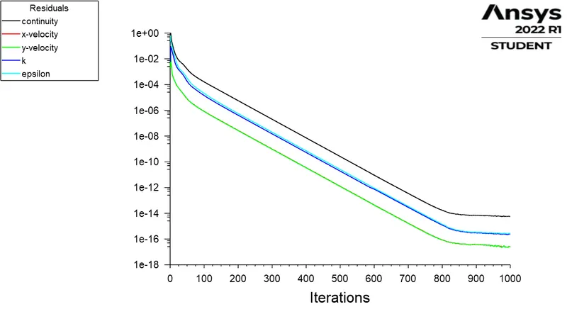
We run the simulation wit Courant number 10 and for 1000 iterations.
Result:
Resuidal -
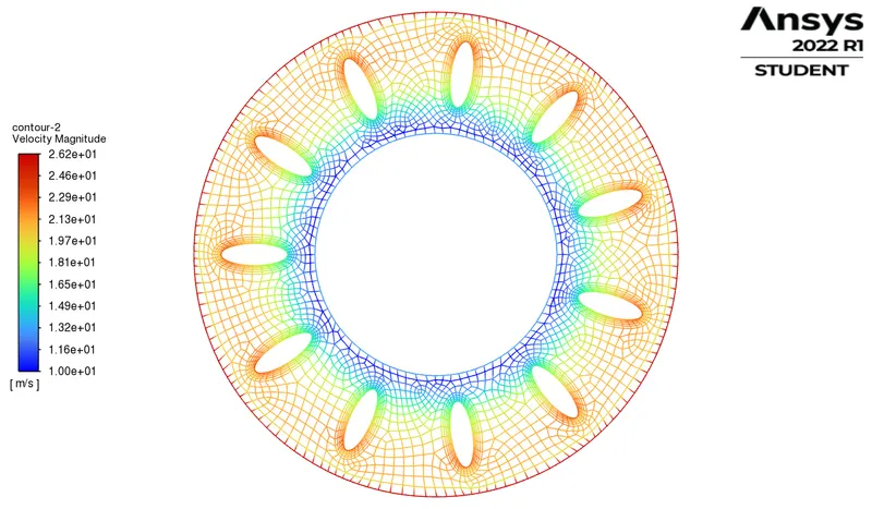
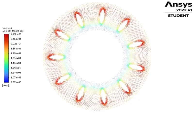
Velocity -
Pressure -
Conclusion:
The velocity of 229 m/s is maximum at the outer frame or at the walls and along the tip of the air-foils. and the velocity decreases as moved towards the center of the rotor.