Week 4 - CHT Analysis on Exhaust port
Aim:
To do a Conjucate Heat Transfer analysis of an exhaust port. We then find the heat transfer Co-Efficient along the walls of the outlet.
Introduction :
Conjugate Heat Transfer or CHT is a type of heat transfer analysis between solid and fluid,the type of heat transfer can be convection , conduction or both. This process depends on change in temperature of two bodies therefor the rate of heat transfer is directily propotional to the change in temperature. It is specifically mentioned as conjucate, because the transfer of heat is a combination of both convection and conduction process. In industrial purpous computer chip, mechanical parts,turbines and other components needs to be designed robust for effective use under extreme conditions this is the reason why the combination of both process is considered, as in both forced and normal convection fluid always surrounds the solid body. They have wide range of applications from aircraft,engines and Heat exchangers to chip, Food storage containers and radiators. The theoratical way to calculate Nusselt number is ,
Nu = hl/k
h= conductive heat transfer [W/m2.K]
l = Characteristic Length (m)
k = Thermal Conductivity [W/m.K]
Modelling and Setup:
In this problem we will be solving for a basic Exhaust port with four Inlets and one Outlet with Inlet velocity of 5 m/s at a temperature of 700 K. In our case we know the the outerwall convection between the exhaust port to the atmospheric air as 20 and our aim is to get the heat transfer Co-Efficient at the Inner wall of the exhaust port as conduction , by this valus we can predict the maximum heat transfer between air and the Exhaust port made up of Aluminium.
The model is imported to space claim
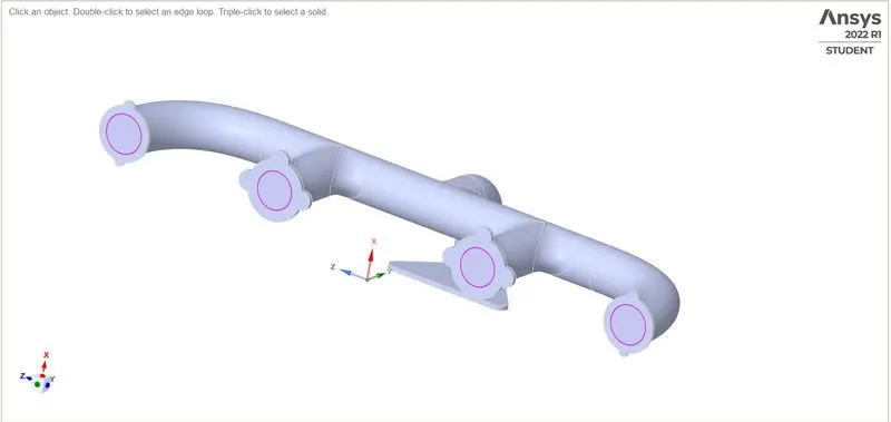
Since our aim is to only capture the inner wall results we split the inner air-solid wall Interactions as fluid volume and we select share topology for sharing the data flow between two bodies.
Procedure:
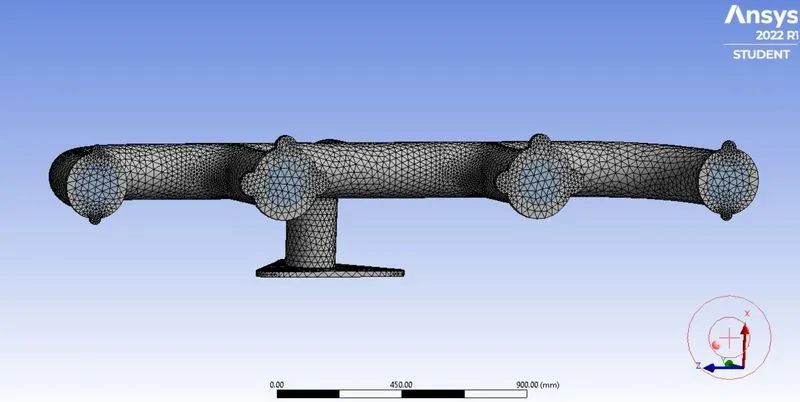
- We initially create a bese line Simulation for the exhaust port with the default Mesh size. For this a mesh size of 150 mm is set,both the bodies are set to same mesh size.
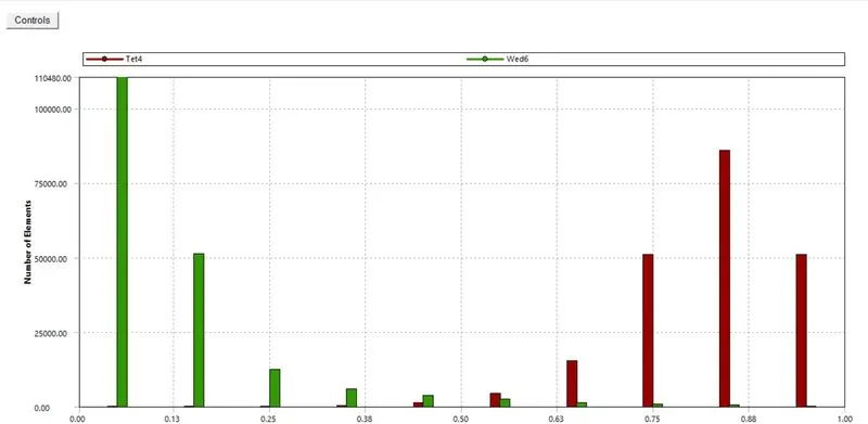
Final Mesh Quality after Refinement
- Then for the further cases we add Inflation Layers and Mesh Sizing. Since it is a Turbulance model we choose either of K-epsilon or K-omega model. For both current setup and for refined mesh case we choose K-epsilon model base on the model we choose the Y+ value changes accordingly and thus changing the total layer thickness for the inflation layers. Since this is a k-epsilon model the value of Y+ should be greater than 50 ,accordingly the total thickness for this model is 5 mm and this will be throughout the walls of the created Fluid Volume of the model.
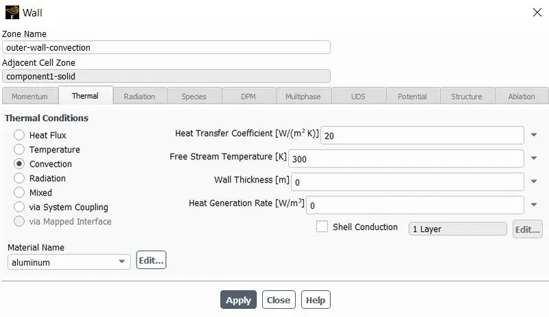
- We open the setup to initialize and add boundary conditions. We also need to calculate the energy equation,then we choose te required viscous model as mentioned previously. For the Inlet conditions we give 5 m/s as the Inlet velocity of Hot air at 700 K and the Heat Transfer Co-Efficient for Aluminium is 20 W/(m2 K) is given for Outer wall convection.
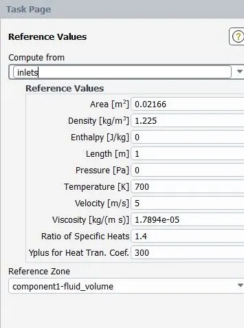
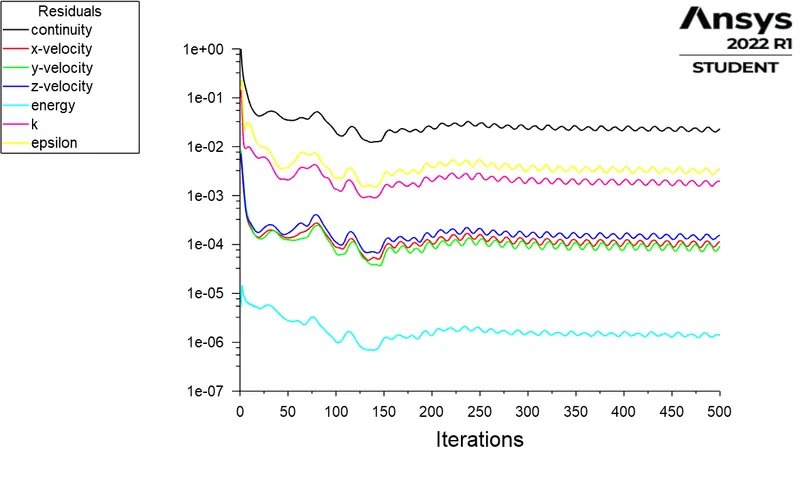
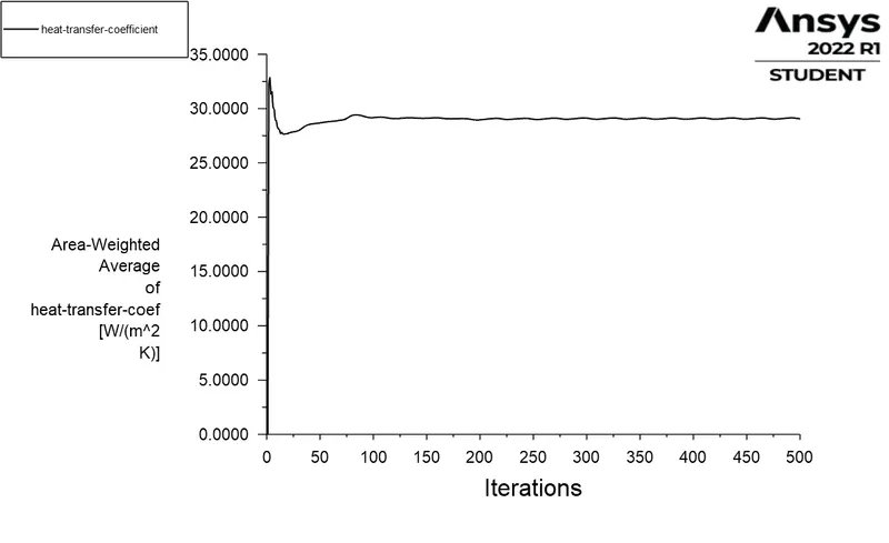
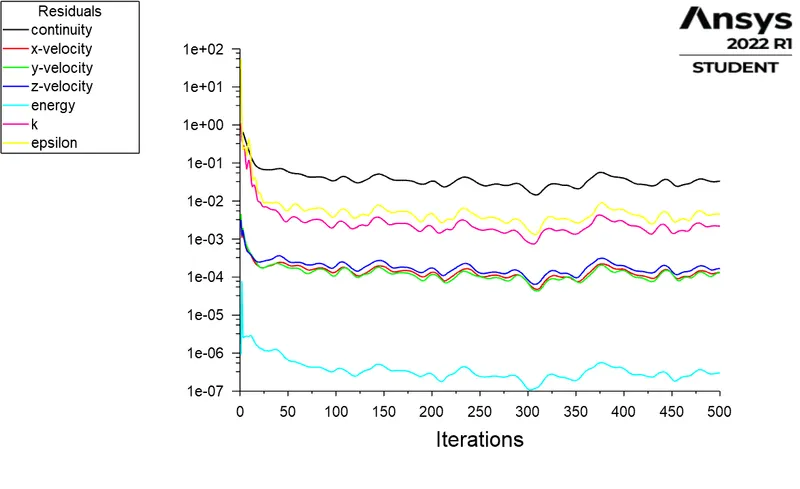
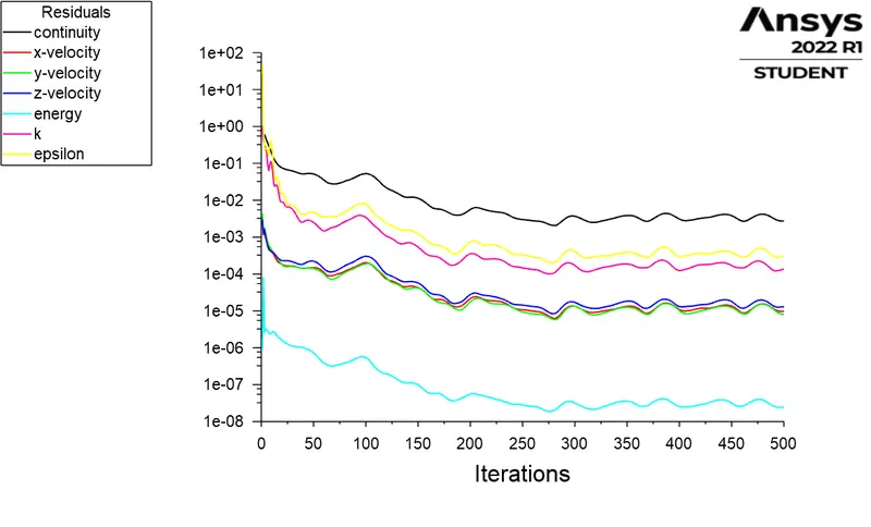
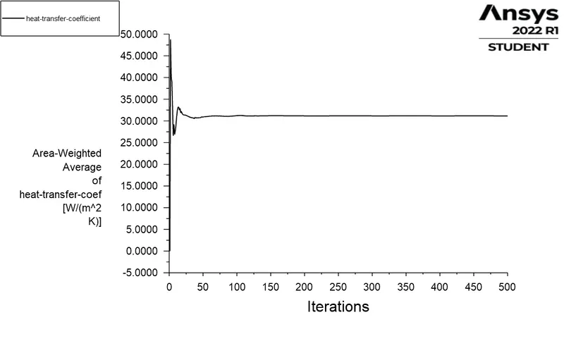
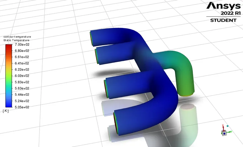
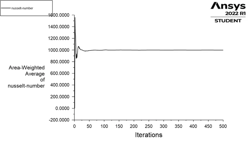
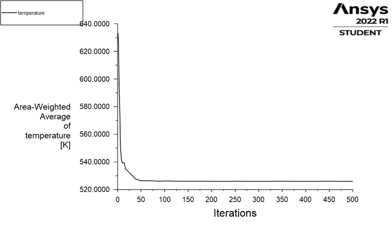
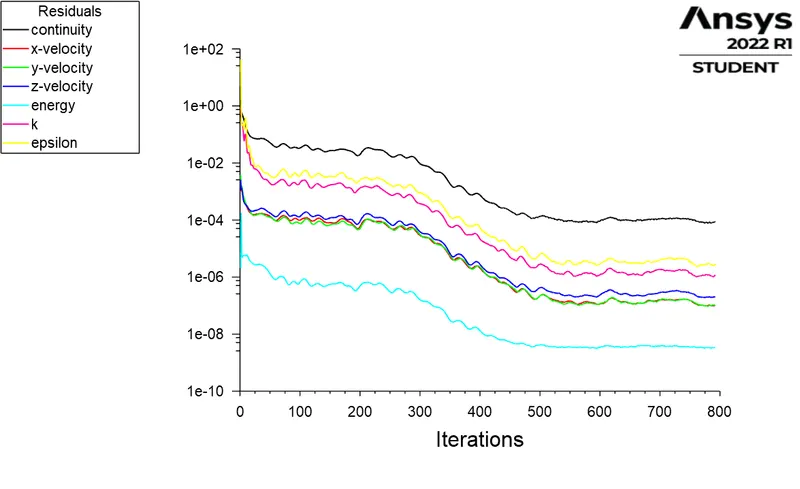
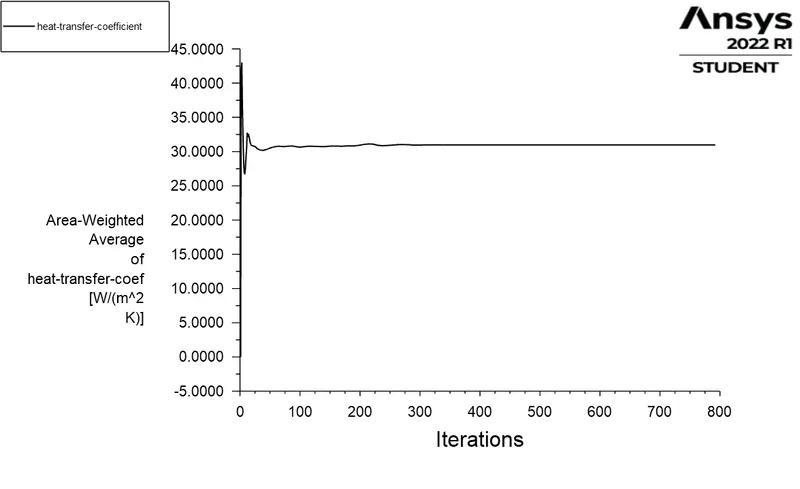
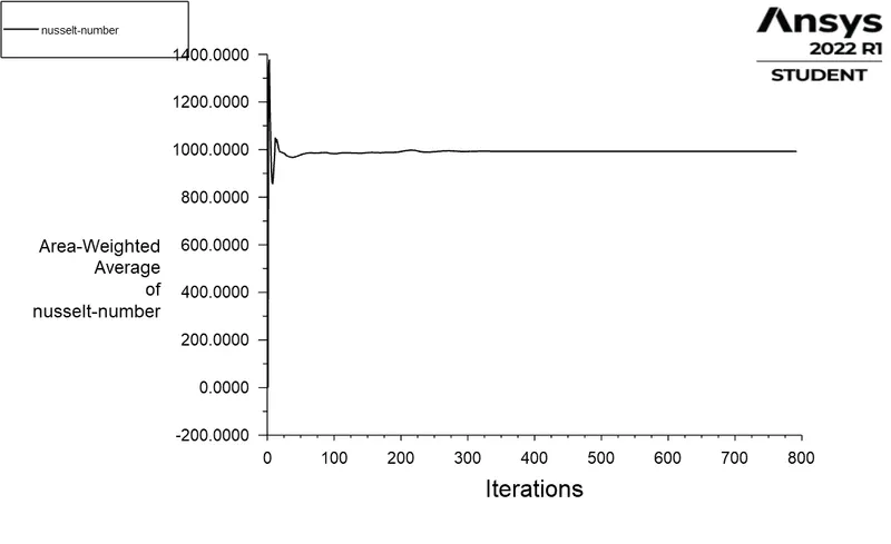
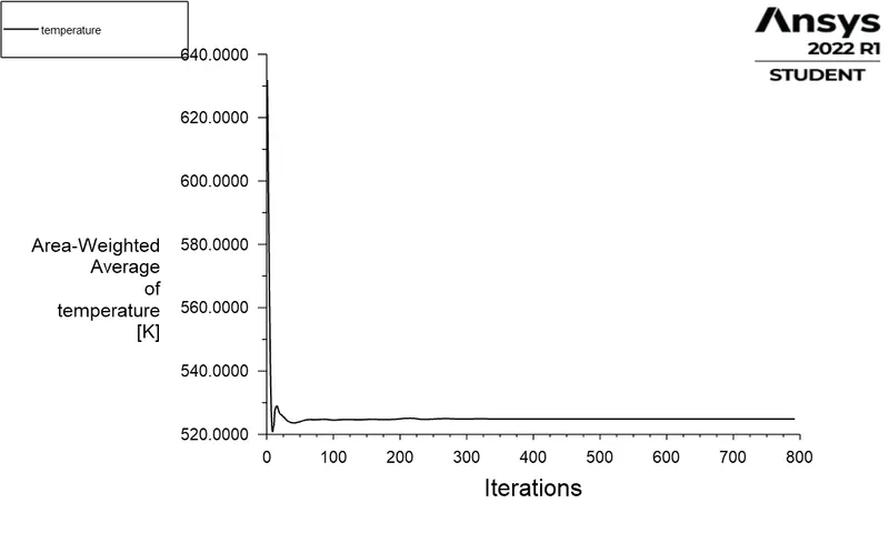
- Then we give the Referance value from the Inlet and the overall length of the Exhaust mainfold is given as 1 and and the area is calculated from the radius of the inlet port. We then add two plots to find area weighted average of Heat transfer Co-efficient or Flim Effectivness , the average temperature at the Outlet and Nusselt Number. The Nusselt number for a turbulance model between 100-1000 means the heat transfer by convection is done effectively. Then we Initialze the equation and create temperature contour and run till Convergence is acheived.
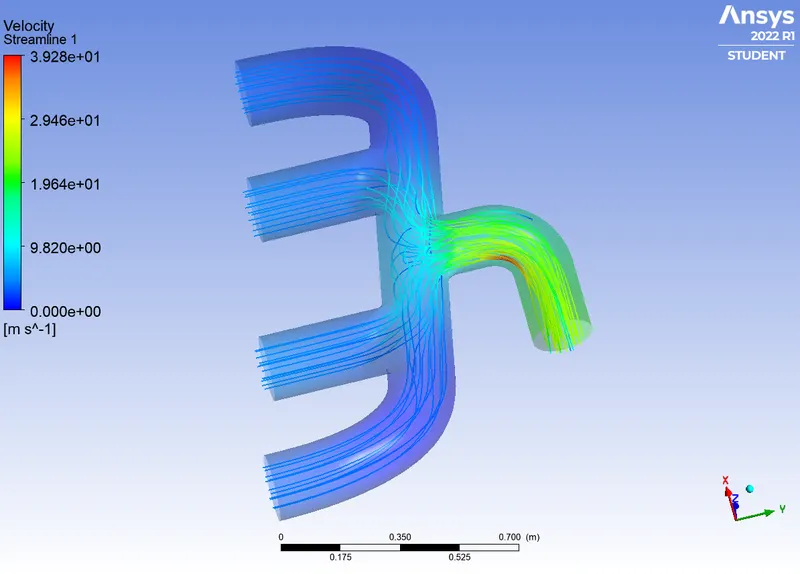
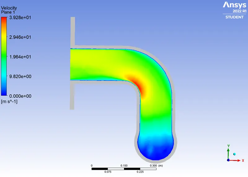
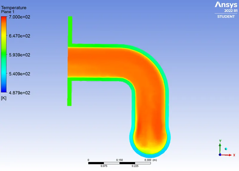
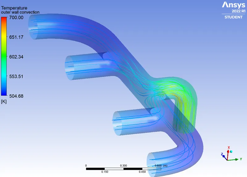
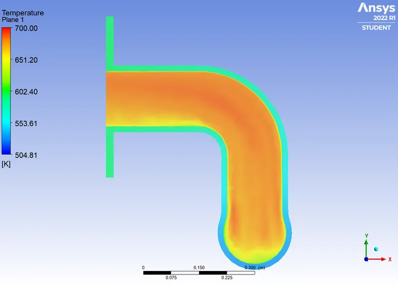
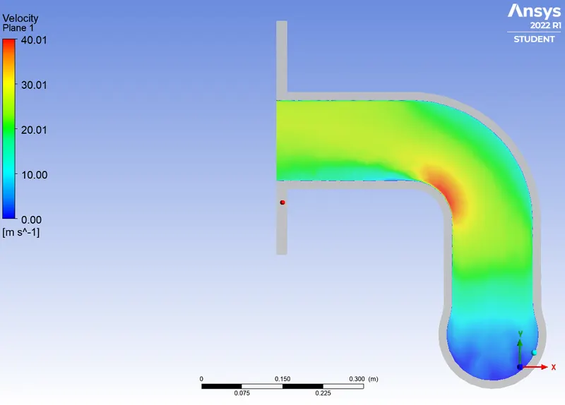
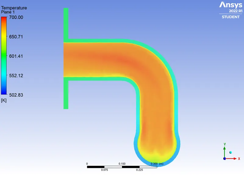
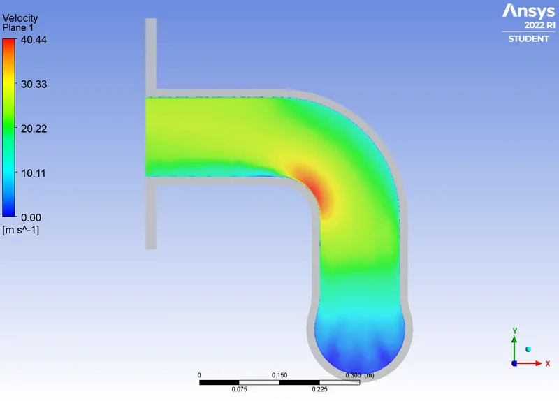
- We then Open CFD-Post to visuzlize the Velocity,temperature, and Heat transfer Coefficient along the Exhaust port and at the outlet.
Baseline Simulation:
Mesh Size: 150 mm
No.of Elements: 203656
Inflation Layers: NIL
Heat Transfer Coefficient: 29.061021 W/(m2 K)
Nusselt Number: 931.25118
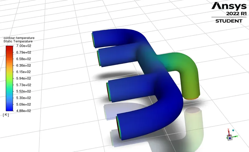
Average Temperature: 515.77019 K
Mesh Independet Study:
Refined Mesh Conditions:
Mesh Size Solid Volume: 150 mm
Mesh Size Fluid Volume: 90 mm
No.of Elements: 241287
Inflation Layers: 6
Total Thickness: 5 mm
Heat Transfer Coefficient: 31.305972 W/(m2 K)
Nusselt Number: 1003.1918
Average Temperature: 526.019 K
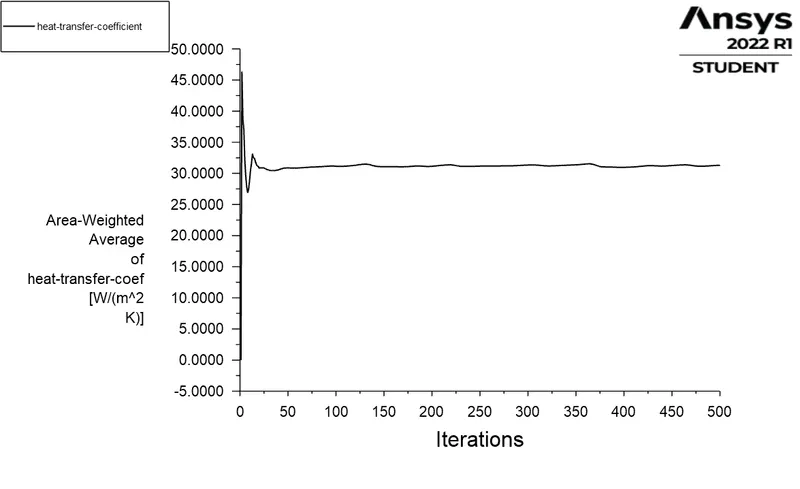
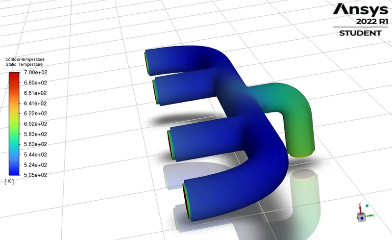
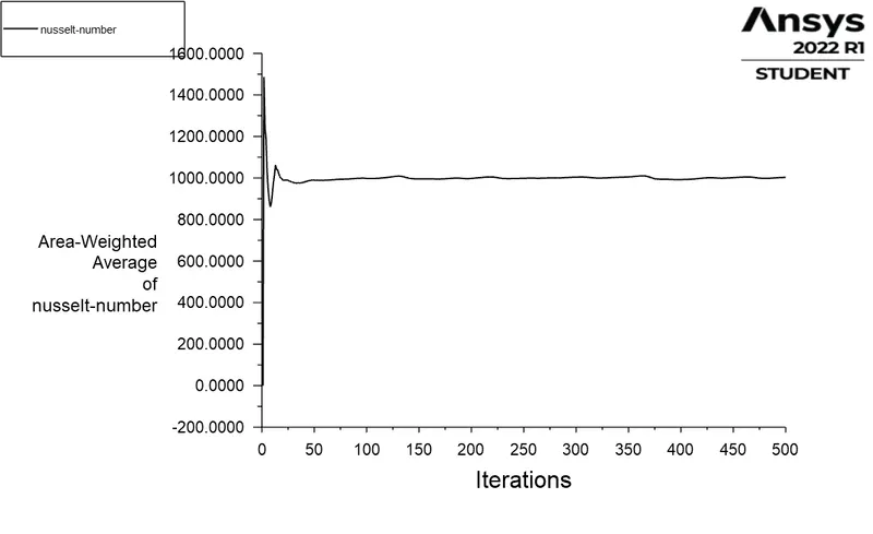
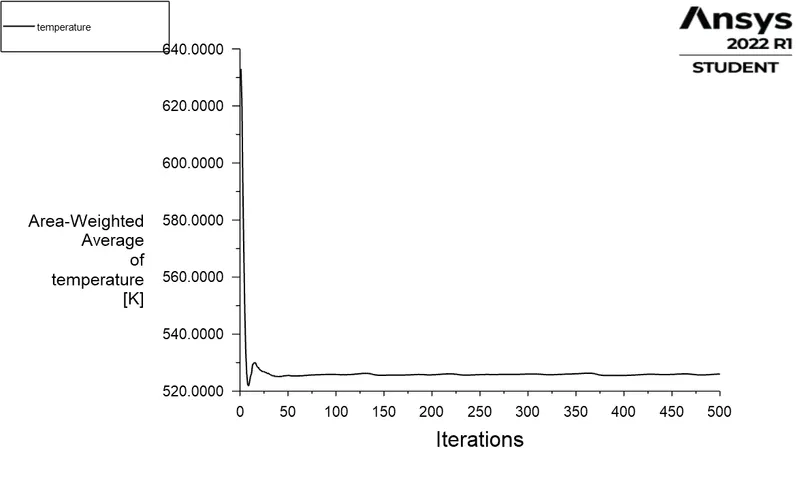
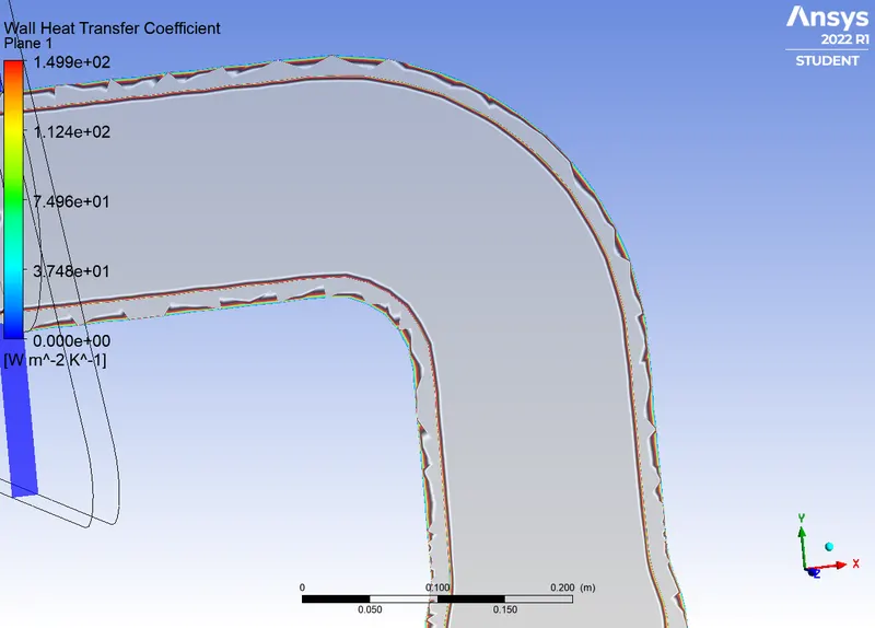
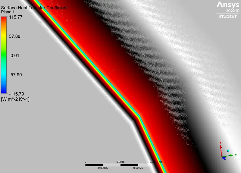
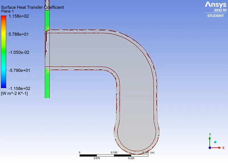
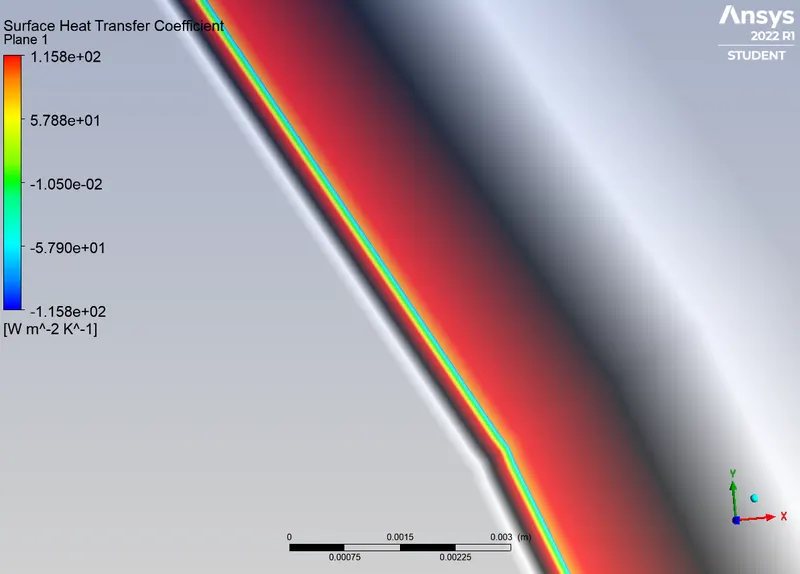
Since we only calculated the Heat transfer coefficient along the walls and excluded the vloume beyond the wall region the contour plot is thin.
Mesh Size Solid Volume: 150 mm
Mesh Size Fluid Volume: 50mm
No.of Elements: 295767
Inflation Layers: 6
Total Thickness: 5 mm
Heat Transfer Coefficient: 31.14664 W/(m2 K)
Nusselt Number: 998.1005
Average Temperature: 525.9794 K
Mesh Size Solid Volume: 60 mm
Mesh Size Fluid Volume: 20 mm
No.of Elements: 396807
Inflation Layers: 6
Total Thickness: 5 mm
Heat Transfer Coefficient:30.905019 W/(m2 K)
Nusselt Number: 990.55871
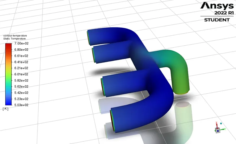
Average Temperature: 524.9288 K
Conclusion:
| S.No | Mesh Size(mm) | Inflation (mm) | No.of Elements |
Heat Transfer Co-Efficient (W/(m2 K)) |
Outlet Temperature (K) |
Nusselt Number |
| 1 | 150 | NIL | 203656 | 29.061021 | 515.770 | 931.25118 |
| 2 | 150 & 90 | 5 | 241287 | 31.305972 | 526.019 | 1003.1918 |
| 3 | 150 & 50 | 5 | 295767 | 31.14664 | 525.979 | 998.1005 |
| 4 | 60 & 20 | 5 | 396807 | 30.905019 | 524.92886 | 990.55871 |
The change in Heat transfer Co-Efficeint is less than 0.6 for the final two value, therefore the HTC is 30.905 W/(m2.K). The results clearly shows that the accuracy of HTC value as we refine the mesh and add Inflation layers to the model. Therefore apart from external factors affecting the results the HTC while simulating depends on two majour things the Y+ value and the corresponding Turbulance model. The mesh size should not exceed a certain limit as too much refinement will have less significant and consumes more time for simulating ,so thats why we need to do mesh independent test to decide the exact refinement required for a paticular model.
As Mentioned earlier the k-omega (1<= Y+ <= 30) is used when we have to capture the near wall turbulance of a model and K-epsilon
( 50<= Y+ <= 300) will be when the turbulant effect is away from the wall.
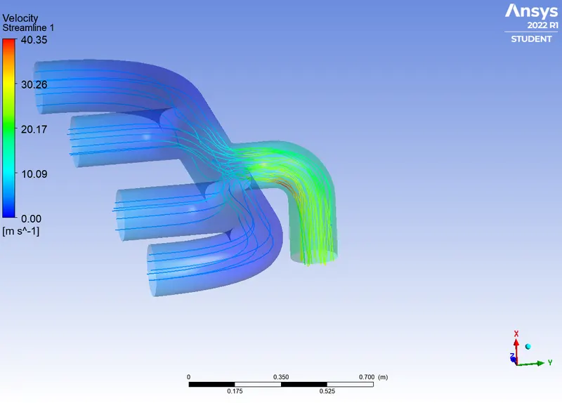
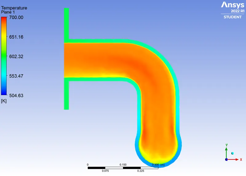
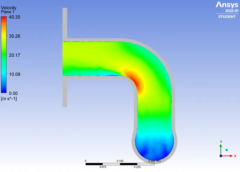
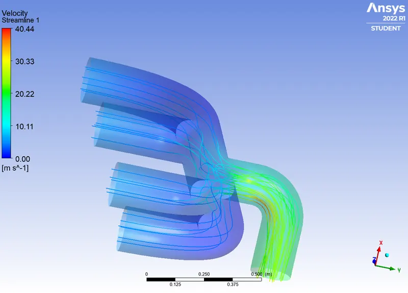
Further we can inffer from the velocity contour at the outlet port that along the bend of the exhaust port the velocity increase and this is due to the curvature and the velociy from four inlet port is chhannled throuh a single outlet port this increase the velocity and the temperature greater than any other region in the Exhaust mainfold. The increse in velocity results in Increase in Reynolds Number. Thus the heat transfer co-efficient is high and that means more heat is transfer takes at that place thus the interaction between solid body and fluid is high at that palce.
To conclude by simulating for the exhaust port i learned how to do a CHT analysis on a given module and cou inffer from the results obtained.