Week 7 - Simulation of a 1D Super-sonic nozzle flow simulation using Macormack Method

The numerical solution of isentropic flow of a quasi 1-D subsonic - supersonic nozzel does not have any meaning. Instead of representaing the analytical solution in an approximated form we try to use CFD in various streams. In this case we apply CFD for a numerical solution with conservative and non-conservative forms.

Conservative Form:

Contunity Equation = `(delp')/(delt') = rho'(delV')/(delx') - rho'V' (del(ln A))/(delx') - V'(delp')/(delx')`

Momentum Equation = `(delV')/(delt')= V' (delV')/(delx') - 1/gamma ((delT')/(delx') +(T')/(rho') (delrho')/(delx'))`

Energy Equation = `(delT')/(delt') = V'(delT')/(delx') - (gamma - 1)T'((delV')/(delx') +V'(delln(A'))/(delx'))`

Non-Conservative Form:

Contunity Equation = `(del( rho'A'))/(delt') + (del( rho'A'V'))/(delx') = 0`

Momentum Equation = `(del( rho'A'V'))/(delx') + ((del( rho'A'V ' ^2) +((1/gamma)(p'A')))/(delx'))=(1/gamma) p' (delA')/(delx')`

Energy Equation = `(del(rho'((T')/(gamma-1) +gamma/2 V'^2)A'))/(delt') + (del((rho'((T')/(gamma-1) +gamma/2 V'^2)V'A')+p'A'V'))/(delx') = 0`

Non-Dimentional Quantities:

Temperature : `T'=T/(To)`

Pressure : `P'=P/(Po)`

Distance : `x'=x/L`

Velocity : `V'=V/(ao)`

Time : `t'=t/(L/(ao))`

Area : `A'=A/(Astar)`

MacCarmack Method:

We use this method to descritize the numerical solution. It involves two steps Predictor and corrector step.

Predictor step - The value 'U' ant time 'n+1' is obtained by replacing the spatial and temporal derivatives in the previous first order equation using Forward difference.

Correctod step - In this step the value 'U' found in predictor step is corrected according to the equation ,by using Backward difference scheme. The time step is used as `(Deltat)/2`.

Main Function:

clear all 
close all
clc
%input parameters
n=31;
gamma = 1.4;
x=linspace(0,3,n);
dx=x(2)-x(1);

nt=1500;
c=0.5;

%Non-Conservative Form
tic;
[Mass_flowrate_NC,Pressure_NC,Machnumber_NC,rho_NC,v_NC,T_NC,rho_throat_NC,v_throat_NC,T_throat_NC,Massflowrate_throat_NC,Pressure_throat_NC,machnumber_throat_NC]=NonConservation(x,dx,n,gamma,nt,c);
Time1=toc;
fprintf('Total time Non-Conservative Form; %0.4f',Time1);
hold on

figure(2)

%density
subplot(4,1,1)
plot(linspace(1,nt,nt),rho_throat_NC,'Color','m')
ylabel('Density')
legend({'Density at throat'});
axis([0 1500 0 1.3]);
grid minor;
title('Timestep verification at throat (NC)')

%Temperature
subplot(4,1,2)
plot(linspace(1,nt,nt),T_throat_NC,'Color','c')
ylabel('Temperature')
legend({'Temperature at throat'});
axis([0 1500 0.6 1]);
grid minor;

%pressure
subplot(4,1,3)
plot(linspace(1,nt,nt),Pressure_throat_NC,'Color','g')
ylabel('Pressure')
legend({'Pressure at throat'});
axis([0 1500 0.4 1.1]);
grid minor;

%Mach Number
subplot(4,1,4)
plot(linspace(1,nt,nt),machnumber_throat_NC,'Color','y')
xlabel('Timestep')
ylabel('Mach Number')
legend({'Machnumber at throat'});
axis([0 1500 0.6 1.4]);
grid minor;

figure(3);

%Density
subplot(4,1,1)
plot(x,rho_NC,'Color','m')
ylabel('Density')
legend({'Density at throat'});
axis([0 3 0 1]);
grid minor;
title('Variation of Flow rate Distribution (NC)')

%Temperature
subplot(4,1,2)
plot(x,T_NC,'Color','c')
ylabel('Temperature')
legend({'temperature at throat'});
axis([0 3 0 1]);
grid minor;

%Pressure
subplot(4,1,3)
plot(x,Pressure_NC,'Color','g')
ylabel('Pressure')
legend({'Pressure at throat'});
axis([0 3 0 1]);
grid minor;

%Mach Number
subplot(4,1,4)
plot(x,Machnumber_NC,'Color','y')
xlabel('Nozzle Length')
ylabel('Mach Number')
legend({'Mach Number'});
axis([0 3 0 4]);
grid minor;

%Conservation Form
tic;
[Mass_flowrate_C,Pressure_C,Machnumber_C,rho_C,v_C,T_C,rho_throat_C,v_throat_C,T_throat_C,Massflowrate_throat_C,Pressure_throat_C,machnumber_throat_C]=Conservation(x,dx,n,gamma,nt,c);
Time2=toc;
fprintf('Total time Conservative Form; %0.4f',Time2);

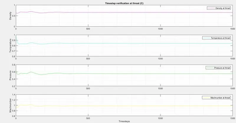
figure(5)

%density
subplot(4,1,1)
plot(rho_throat_C,'Color','m')
ylabel('Density')
legend({'Density at throat'});
axis([0 1500 0 1]);
grid minor;
title('Timestep verification at throat (C)')

%Temperature
subplot(4,1,2)
plot(T_throat_C,'Color','c')
ylabel('Temperature')
legend({'Temperature at throat'});
axis([0 1500 0.6 1]);
grid minor;

%pressure
subplot(4,1,3)
plot(Pressure_throat_C,'Color','g')
ylabel('Pressure')
legend({'Pressure at throat'});
axis([0 1500 0.2 0.8]);
grid minor;

%Mach Number
subplot(4,1,4)
plot(machnumber_throat_C,'Color','y')
ylabel('Machnumber')
xlabel('Timesteps')
legend({'Machnumber at throat'});
axis([0 1500 0.6 1.4]);
grid minor;

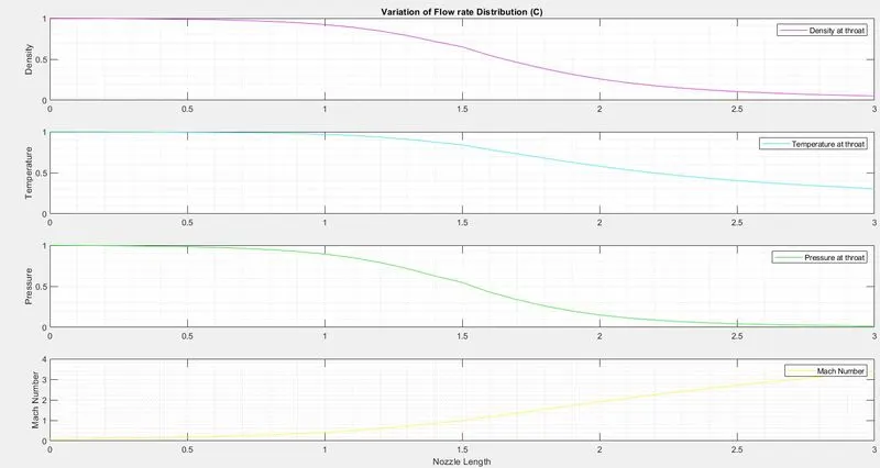
figure(6);

%Density
subplot(4,1,1)
plot(x,rho_C,'Color','m')
ylabel('Density')
legend({'Density at throat'});
axis([0 3 0 1]);
grid minor;
title('Variation of Flow rate Distribution (C)')

%Temperature
subplot(4,1,2)
plot(x,T_C,'Color','c')
ylabel('Temperature')
legend({'Temperature at throat'});
axis([0 3 0 1]);
grid minor;

%Pressure
subplot(4,1,3)
plot(x,Pressure_C,'Color','g')
ylabel('Pressure')
legend({'Pressure at throat'});
axis([0 3 0 1]);
grid minor;

%Mach Number
subplot(4,1,4)
plot(x,Machnumber_C,'Color','y')
xlabel('Nozzle Length')
ylabel('Mach Number')
legend({'Mach Number'});
axis([0 3 0 4]);
grid minor;

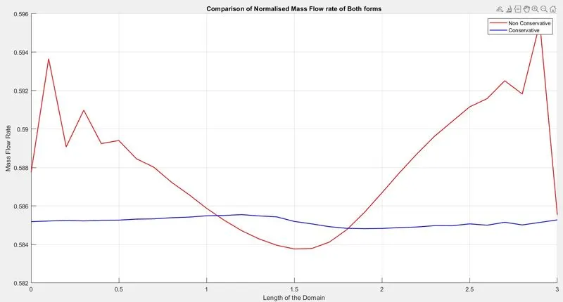
figure(7)
hold on
plot(x,Mass_flowrate_NC,'r','linewidth',1.25)
hold on;
plot(x,Mass_flowrate_C,'b','linewidth',1.25)
hold on;
grid on

legend('Non Conservative','Conservative');
xlabel('Length of the Domain')
ylabel('Mass Flow Rate')
title('Comparison of Normalised Mass Flow rate of Both forms')

Explanation:

1.The initial conditions for Density,Temperature,velocity are defined.

2. The grid space is created and the values for constants are initialised and the area profile is created.

3.The for loop is created which runs for given time steps, and it solves the governing equations using the above mentioned technique.

4.For Conservative form alone solution vector 'U' ,Flux vector 'F' and Source Term 'J'.

4.Thereby both Predictor and Corrector steps are calculated seperatly inside two different loops.

5.The old values are updated after each timestep.

6.Finally the two values for density ,velocity and tempearture is averaged .

7.Both boundary and exit conditions are computed and Massflow rate,Pressure, Mach number values are obtained at throat as well.

8.And the graph Distance vs Mass flow rate is plotted.

Non-Conservative Form Function:

function [Mass_flowrate_NC,Pressure_NC,Machnumber_NC,rho_NC,v_NC,T_NC,rho_throat_NC,v_throat_NC,T_throat_NC,Massflowrate_throat_NC,Pressure_throat_NC,machnumber_throat_NC]=NonConservation(x,dx,n,gamma,nt,c)

%Initialising
rho_NC= 1- 0.3146*x;
T_NC= 1 - 0.2341*x;
v_NC= (0.1 +1.09*x).*T_NC.^0.5;
a= 1+ 2.2*(x-1.5).^2;
throat=find(a==1);

for k = 1:nt
    dt=min(c.*dx./(sqrt(T_NC)+ v_NC));
    rho_old =rho_NC;
    T_old = T_NC;
    v_old = v_NC;

    %predictor step
    for j= 2:n-1
        dv_dx = (v_NC(j+1) - v_NC(j))/dx;
        drho_dx = (rho_NC(j+1) - rho_NC(j))/dx;
        dT_dx = (T_NC(j+1) - T_NC(j))/dx;
        dloga_dx = (log(a(j+1)) - log(a(j)))/dx;
     
        drho_dt_P(j)= -rho_NC(j)*dv_dx - rho_NC(j)*v_NC(j)*dloga_dx - v_NC(j)*drho_dx;
        dv_dt_P(j)= -v_NC(j)*dv_dx - (1/gamma)*(dT_dx + ( T_NC(j)*drho_dx/rho_NC(j)));
        dT_dt_P(j)= -v_NC(j)*dT_dx - (gamma -1)*T_NC(j)*(dv_dx + v_NC(j)*dloga_dx);

        %solution Update
        rho_NC(j) = rho_NC(j) + drho_dt_P(j)*dt;
        v_NC(j) = v_NC(j) + dv_dt_P(j)*dt;
        T_NC(j) = T_NC(j) + dT_dt_P(j)*dt;

    end

    %Corrector Method
    for j = 2:n-1

        dv_dx = (v_NC(j) - v_NC(j-1))/dx;
        drho_dx = (rho_NC(j) - rho_NC(j-1))/dx;
        dT_dx = (T_NC(j) - T_NC(j-1))/dx;
        dloga_dx = (log(a(j)) - log(a(j-1)))/dx;
     
        drho_dt_C(j)= -rho_NC(j)*dv_dx - rho_NC(j)*v_NC(j)*dloga_dx - v_NC(j)*drho_dx;
        dv_dt_C(j)= -v_NC(j)*dv_dx - (1/gamma)*(dT_dx + ( T_NC(j)*drho_dx/rho_NC(j)));
        dT_dt_C(j)= -v_NC(j)*dT_dx - (gamma -1)*T_NC(j)*(dv_dx + v_NC(j)*dloga_dx);

    end

    drho_dt= 0.5.*(drho_dt_P + drho_dt_C);
    dv_dt= 0.5.*(dv_dt_P + dv_dt_C);
    dT_dt= 0.5.*(dT_dt_P + dT_dt_C);

    %Final Update
    for i = 2:n-1
        rho_NC(i) = rho_old(i) + drho_dt(i)*dt;
        v_NC(i) = v_old(i) + dv_dt(i)*dt;
        T_NC(i) = T_old(i) + dT_dt(i)*dt;

    end

    %BC's
    rho_NC(1) = 1;
    v_NC(1) = 2*v_NC(2) - v_NC(3);
    T_NC(1) = 1;

    %outlet
    rho_NC(n) = 2*rho_NC(n-1) - rho_NC(n-2);
    v_NC(n) = 2*v_NC(n-1) - v_NC(n-2);
    T_NC(n) = 2*T_NC(n-1) - T_NC(n-2);

    Mass_flowrate_NC = rho_NC.*a.*v_NC;
    Pressure_NC = rho_NC.*T_NC;
    Machnumber_NC = (v_NC./sqrt(T_NC));

    rho_throat_NC(k) = rho_NC(throat);
    T_throat_NC(k) = T_NC(throat);
    v_throat_NC(k) = v_NC(throat);
    Massflowrate_throat_NC(k) = Mass_flowrate_NC(throat);
    Pressure_throat_NC(k) = Pressure_NC(throat);
    machnumber_throat_NC(k) = Machnumber_NC(throat);

    %plot
    figure(1)
        if k==50
            plot(x,Mass_flowrate_NC,'m','LineWidth',1.25);
            hold on
        elseif k==100
             plot(x,Mass_flowrate_NC,'c','LineWidth',1.25);
             hold on
        elseif k==200
             plot(x,Mass_flowrate_NC,'g','LineWidth',1.25);
             hold on
        elseif k==400
             plot(x,Mass_flowrate_NC,'y','LineWidth',1.25);
             hold on
        elseif k==800
             plot(x,Mass_flowrate_NC,'k','LineWidth',1.25);
             hold on
        end

        title('Mass flow rates at different Timesteps (NC)')
        xlabel('Distance')
        ylabel('Mass Flow rate')
        legend({'50^t^h Timestep','100^t^h Timestep','200^t^h Timestep','400^t^h Timestep','800^t^h Timestep'})
        axis([0 3 0 2])
        grid on
end
end

Conservative Form Function:

function [Mass_flowrate_C,Pressure_C,Machnumber_C,rho_C,v_C,T_C,rho_throat_C,v_throat_C,T_throat_C,Massflowrate_throat_C,Pressure_throat_C,machnumber_throat_C]=Conservation(x,dx,n,gamma,nt,c)
for i =1:n
    if (x(i) >= 0 && x(i) <= 0.5)
        rho_C(i) = 1;
        T_C(i) = 1;
    elseif (x(i) >= 0.5 && x(i) <= 1.5)
        rho_C(i) = 1 - 0.366*(x(i) - 0.5);
        T_C(i) = 1 - 0.167*(x(i) - 0.5);
    elseif (x(i) >= 1.5 && x(i) <= 3)
        rho_C(i) = 0.634 - 0.3879*(x(i) - 1.5);
        T_C(i) = 0.833 - 0.3507*(x(i) - 1.5);
    end

end

a = 1 + 2.2*(x - 1.5).^2;
throat = find(a==1);

v_C = 0.59./(rho_C.*a);
Pressure_C = rho_C.*T_C;

%Initial solution
U1 = rho_C.*a;
U2 = rho_C.*a.*v_C;
U3 = rho_C.*a.*(T_C./(gamma - 1)) + ((gamma/2).*v_C.^2);

for k=1:nt
    dt = min(c.*dx./(sqrt(T_C) + v_C));

    %Initializing old values
    U1_old = U1;
    U2_old = U2;
    U3_old = U3;

    %Flux vector
    F1 = U2;
    F2 = ((U2.^2)./U1) + ((gamma - 1)/gamma)*(U3 - (gamma/2)*((U2.^2)./U1));
    F3 = ((gamma*U2.*U3)./U1) - (gamma*(gamma - 1)*((U2.^3)./(2*U1.^2)));

    %Predictor
    for j=2:n-1
        J2(j) = (1/gamma)*rho_C(j)*T_C(j)*((a(j+1) - a(j))/dx);

        %contunity
        dU1_dt_P(j) = -((F1(j+1) - F1(j))/dx);

        dU2_dt_P(j) = -((F2(j+1) - F2(j))/dx) +J2(j);

        dU3_dt_P(j) = -((F3(j+1) - F3(j)) / dx);

        %Updating New values
        U1(j) = U1(j) + dU1_dt_P(j)*dt;
        U2(j) = U2(j) + dU2_dt_P(j)*dt;
        U3(j) = U3(j) + dU3_dt_P(j)*dt;
    end

        %updating values
        F1 = U2;
        F2 = ((U2.^2)./U1) + ((gamma - 1)/gamma)*(U3 - ((gamma*0.5*(U2.^2))./(U1)));
        F3 = ((gamma*U2.*U3)./U1) - ((gamma*0.5*(gamma - 1)*(U2.^3))./(U1.^2));

        %Corrector
        for j=2:n-1
            J2(j) = (1/gamma)*rho_C(j)*T_C(j)*((a(j) - a(j-1))/dx);

            %contunity
            dU1_dt_C(j) = -((F1(j) - F1(j-1))/dx);

            dU2_dt_C(j) = -((F2(j) - F2(j-1))/dx) +J2(j);

            dU3_dt_C(j) = -((F3(j) - F3(j-1)) / dx);
        end
        dU1_dt = 0.5*(dU1_dt_P + dU1_dt_C);
        dU2_dt = 0.5*(dU2_dt_P + dU2_dt_C);
        dU3_dt = 0.5*(dU3_dt_P + dU3_dt_C);

        %final Update
        for i= 2:n-1
            U1(i) = U1_old(i) + dU1_dt(i)*dt;
            U2(i) = U2_old(i) + dU2_dt(i)*dt;
            U3(i) = U3_old(i) + dU3_dt(i)*dt;
        end

        %BC's
        U1(1) = rho_C(1)*a(1);
        U2(1) = 2*U2(2) - U2(3);
        v_C(1) = U2(1)./U1(1);
        U3(1) = U1(1)*((T_C(1)/(gamma - 1)) + ((gamma/2)*(v_C(1)).^2));

        %Exit
        U1(n) = 2*U1(n-1) - U1(n-2);
        U2(n) = 2*U2(n-1) - U2(n-2);
        U3(n) = 2*U3(n-1) - U3(n-2);

        rho_C = U1./a;
        v_C = U2./U1;
        T_C = (gamma - 1)*((U3./U1 - (gamma/2)*(v_C).^2));

        %Defining 
        Mass_flowrate_C = rho_C.*a.*v_C;
        Pressure_C= rho_C.*T_C;
        Machnumber_C = (v_C./sqrt(T_C));

        %At Thorat
        rho_throat_C(k) = rho_C(throat);
        T_throat_C(k) = T_C(throat); 
        v_throat_C(k) = v_C(throat);
        Massflowrate_throat_C(k) = Mass_flowrate_C(throat);
        Pressure_throat_C(k) = Pressure_C(throat);
        machnumber_throat_C(k) = Machnumber_C(throat);


        %Plot
        figure(4)
        if k==50
            plot(x,Mass_flowrate_C,'m','LineWidth',1.25)
            hold on
        elseif k==100
            plot(x,Mass_flowrate_C,'c','LineWidth',1.25)
            hold on
        elseif k==200
            plot(x,Mass_flowrate_C,'g','LineWidth',1.25)
            hold on
        elseif k==400
            plot(x,Mass_flowrate_C,'y','LineWidth',1.25)
            hold on
        elseif k==800
            plot(x,Mass_flowrate_C,'k','LineWidth',1.25)
            hold on
        end

        %Lablling
        title('Mass flow rates at different Timestep (C)')
        xlabel('Distance')
        ylabel('Mass Flow rate')
        legend({'50^t^h Timestep','100^t^h Timestep','200^t^h Timestep','400^t^h Timestep','800^t^h Timestep'})
        axis([0 3 0.4 1])
        grid on

end
end

Graphs :

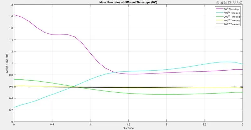
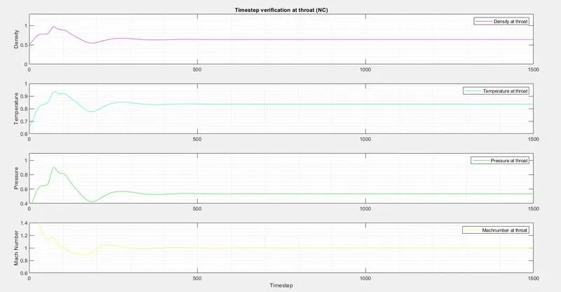
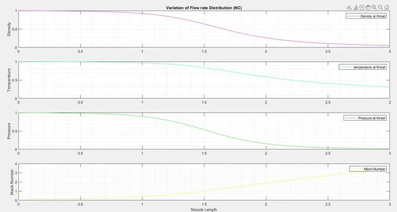
Mass Flow rate using Non-Conservative (NC) approach -

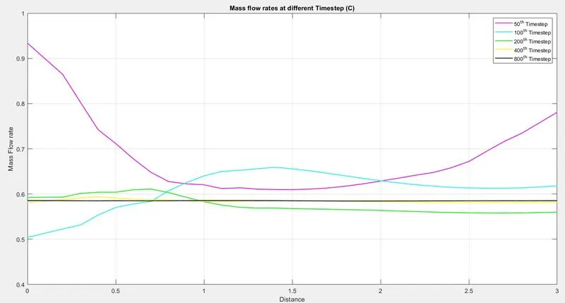
Mass Flow rate using Conservative(C) approach -

Conclusion :

The non-conservative form produces more signifiacnt oscillations than other form. Therefore conservative form requires less number of iterations to obtain steady state condition then Non conservative form.