Week 3.5 - Deriving 4th order approximation of a 2nd order derivative using Taylor Table method

For each type of difference method we have to find the No.of nodes in a stencil to form an equation.

from hint we get that two equations.

P=N-Q+1

P=N-Q

1) Central Difference:

P= order of approximation

N= No.of nodes in stencil

Q= order of derivative

here P is 4 since we require 4th order derivative and Q is 2 since we need the approximation for 2nd order derivative.

4=N-2+1

N=5

we need to conside 5 nodes for the equation and since its a Central difference we need two poins on either side of the reference point f(i). so, we take (i-2) ,(i-1), (i), (i+1), (i+2) as the points.

`del`^2f/`del`x^2 = a f(i-2)+b f(i-1)+c f(i)+d f(i+1)+b f(i+2)`

as we write the taylor equation for each term,

`a f(i-2) =a[ f(i) - f'(i) 2x + (f''(i) (2x)^2 ) /2 - (f'''(i) (2x)^3 ) /6 + (f''''(i) (2x)^4 ) /24 - (f'''''(i) (2x)^5 ) /120 + (f''''''(i) (2x)^6 ) /720 - ......]`

after simplyfing the above equation we get,

`a f(i-2) =af(i) - 2af'(i) x +2a (f''(i) x^2 ) - 4a(f'''(i) x^3 ) /3 + 2a(f''''(i) x^4 ) /3 - 4a(f'''''(i) x^5 ) /15 + 4a(f''''''(i) x^6) /45`

simillarly we get the below equations for other points

`b f(i-1) =bf(i) - bf'(i) x +b (f''(i) x^2 )/2 - b(f'''(i) x^3 ) /6 + b(f''''(i) x^4 )/ 24 - b(f'''''(i) x^5 ) /120 + b(f''''''(i) x^6) /720`

`cf(i) = cf(i)`

`d f(i+1) =df(i) + d f'(i) x +d(f''(i) x^2 )/2 + d(f'''(i) x^3 ) /6 + d(f''''(i) x^4 )/24 + d(f'''''(i) x^5 ) /120 + d(f''''''(i) x^6) /720`

`e f(i+2) =ef(i) + 2ef'(i) x +2e (f''(i) x^2 ) +4e(f'''(i) x^3 ) /3 + 2e(f''''(i) x^4 ) /3 + 4e(f'''''(i) x^5 ) /15 + 4e(f''''''(i) x^6) /45`

	f(i)	f'(i)x	f''(i)x^2	f'''(i)x^3	f''''(i)x^4	f'''''(i)x^5	f''''''(i)x^6
af(i-2)	a	-2a	2a	-4a/3	2a/3	-4a/15	4a/45
bf(i-1)	b	-b	b/2	-b/6	b/24	-b/120	b/720
cf(i)	c	0	0	0	0	0	0
df(i+1)	d	d	d/2	d/6	d/24	d/120	d/720
ef(i+2)	e	2e	2e	4e/3	2e/3	4e/15	4e/45
`sum`	0	0	1	0	0	?	?

The sum of equation f''(i) is alone 1 since we are solving for second order derivative and we only take 5 equations as we only have five unknowns.

For finding the values of a,b,c,d,e we write in into this format ,

`[ [1,1,1,1,1], [ -2,-1,0,1,2],[2,0.5,0,0.5,2],[-1.333,-0.166,0,0.166,1.333],[0.666,0.0416,0,0.04166,0.666]] [[a],[b],[c],[d]] = [[0],[0],[1],[0],[0]]`

we get ,

a=-0.0833

b=1.3334

c=2.5001

`d=1.334`

e=-0.0833

by substuting each value of variables in each colum and exuating we get,

`'(i) rArr a+b+c+d+e = 0`

since a=e; b=d

`f'(i)=2(-0.0833)-1.333+1.333+2(0.0833) = 0`

`f''(i)= 2(-0.0833)+0.5(-1.333)+0.5(1.333)+2(0.0833) = 0

`f'''(i) = -4(-0.0833)/3 - (1.33/6)+(1.33/6) +4(-0.0833/6) = 0`

f''''(i) = 2/3(-0.0833)+(1.333/24)+(1.333/24)+2/2(-0.0833) = 0

f'''''(i) = -4/15(-0.0833) - (1.333/120)+(1.333/120)+4(0.0833/15) = 0

f'''''(i) = 8a/45 + b/360

as we rewrite the initial eqation as,

`del`^2f/`del`x^2= a f(i-2)+b f(i-1)+c f(i)+d f(i+1)+e f(i+2)` = 0+0+1(f''(i)x^2)+0+0+(f''''''(i)x^6)(8a/45+b/360)`

by dividing the equation by `Delta x^2``

`del`^2f/`del`x^2 = (a f(i-2)+b f(i-1)+c f(i)+d f(i+1)+e f(i+2))/(Delta x^2)` = (f''(i))+(x^4)0`

Therefore the Truncatiom=n error is of Power 4 and this approximation is of 4th order.

And to find the 4th order approximation for a second order derivative can be done by substuting values od a,b,c,d,e in the below equation.

`del`^2f/`del`x^2= (a f(i-2)+b f(i-1)+c f(i)+d f(i+1)+e f(i+2)/ (Delta x^2)``

2) Skewed right-side difference:

P=N-Q

P= order of approximation

N= No.of nodes in stencil

Q= order of derivative

here P is 4 since we require 4th order derivative and Q is 2 since we need the approximation for 2nd order derivative.

4=N-2

N=6

We need to conside 6 nodes for the equation and since its a Skewed right-side difference we need 5 poins on right side of the reference point f(i). so, we take (i), (i+1), (i+2),(i+3),(i+4),(i+5) as the points.

`del`^2f/`del`x^2 = a f(i)+b f(i+1)+c f(i+2)+d f(i+3)+e f(i+4)+g f(i+5)`

as we write the taylor equation for each term,

`c f(i+2) =c[ f(i) + f'(i) 2x + (f''(i) (2x)^2 ) /2 + (f'''(i) (2x)^3 ) /6 + (f''''(i) (2x)^4 ) /24 + (f'''''(i) (2x)^5 ) /120 + (f''''''(i) (2x)^6 ) /720 - ......]`

after simplyfing the above equation we get,

`c f(i+2) =cf(i) + 2c f'(i) x +2c (f''(i) x^2 ) + 4c (f'''(i) x^3 ) /3 + 2c(f''''(i) x^4 ) /3 +4c(f'''''(i) x^5 ) /15 + 4c(f''''''(i) x^6) /45`

simillarly we get the below equations for other points

`b f(i+1) =bf(i) + b f'(i) x +b (f''(i) x^2 )/2 + b(f'''(i) x^3 ) /6 + b(f''''(i) x^4 )/ 24 + b(f'''''(i) x^5 ) /120 + b(f''''''(i) x^6) /720`

`af(i) = af(i)`

`d f(i+3) =d f(i) + 3d f'(i) x +9/2d(f''(i) x^2 ) + 27/6d(f'''(i) x^3 ) +81/24 d(f''''(i) x^4 ) +243/120 d(f'''''(i) x^5 ) + 729/720d(f''''''(i) x^6)`

`e f(i+4) =ef(i) + 4ef'(i) x +8e (f''(i) x^2 ) +64/6e(f'''(i) x^3 ) + 256/24e(f''''(i) x^4 ) + 1024/120 e(f'''''(i) x^5 ) + 4096/720e(f''''''(i) x^6)`

`g f(i+5) =gf(i) + 5gf'(i) x +25/2g (f''(i) x^2 ) +125/6g(f'''(i) x^3 ) + 625/24g(f''''(i) x^4 ) + 3125/120 g(f'''''(i) x^5 ) + 15625/720 g(f''''''(i) x^6`

	f(i)	f'(i)x	f''(i)x^2	f'''(i)x^3	f''''(i)x^4	f'''''(i)x^5	f''''''(i)x^6
af(i)	a	0	0	0	0	0	0
bf(i+1)	b	b	b/2	b/6	b/24	b/120	b/720
cf(i+2)	c	2c	2c	4c/3	2c/3	4c/15	4c/45
df(i+3)	d	3d	9d/2	27d/6	81d/24	81d/40	81d/80
ef(i+4)	e	4e	8e	64e/6	256e/24	128e/15	256e/45
gf(i+5)	g	5g	25g/2	125g/6	625g/24	3125g/120	3125g/144
`sum`	0	0	1	0	0	0	?

The sum of equation f''(i) is alone 1 since we are solving for second order derivative and we only take 6 equations as we only have six unknowns.

For finding the values of a,b,c,d,e,g we write in into this format ,

`[[1,1,1,1,1,1],[0,1,2,3,4,5],[0,1/2,2,9/2,8,25/2],[0,1/6,4/3,27/6,64/6,125/6],[0,1/24,2/3,81/24,256/24,625/24],[0,1/120,4/15,81/40,128/15,3125/120]] [[a],[b],[c],[d],[e],[g]] = [[0],[0],[1],[0],[0],[0]]`

we get ,

a= 3.7500

b=-12.8333

c=17.8333

d=-13.0000

e=5.0833

g=-0.8333

by substuting each value of variables in each colum and exuating we get,

`f(i) rArr a+b+c+d+e=g = 0`

`f'(i)rArr 0-12.8333+2(17.8333) - 3(-13.0000)+4(5.0833) - 5(0.8333)= 0`

`f''(i)rArr 0 -12.8333/2 +2(17.8333) - 9/2(13.0000)+8(5.0833)-25/2(0.8333)=1`

`f'''(i)rArr 0 -12.8333/6 +4/3(17.8333) - 27/6(13.0000)+64/6(5.0833)-125/6(0.8333)= 0`

`f''''(i)rArr 0-(12.8333)/24 + 2/3(17.8333)-81/24(13.0000)+256/24(5.0833)+625/24(-0.8333) = 0`

`f'''''(i) rArr 0 - 12.8333/120+4/15(17.8333)-81/40(13.0000)+128/15(5.0833)-3125/120(0.8333)=0`

`f'''''(i) rArr 0- 12.8333/720+4/45(17.8333)-81/80(13.0000)+256/45(5.08333)-3125/144(0.8333)`

as we rewrite the initial eqation as,

`del`^2f/`del`x^2= a f(i)+b f(i-1)+c f(i-2)+d f(i-3)+e f(i-4)+g f(i-5)` = 0+0+1(f''(i)x^2)+0+0+0+(f''''''(i)x^6)(b/720+4/45c+81/80d+256/45e+3125/144g)`

by dividing the equation by `Delta x^2``

`del`^2f/`del`x^2 = (a f(i)+b f(i+1)+c f(i+2)+d f(i+3)+e f(i+4)+gf(i+5)/(Delta x^2)` = (f''(i))+(x^4)0`

Therefore the Truncatiom=n error is of Power 4 and this approximation is of 4th order.

And to find the 4th order approximation for a second order derivative can be done by substuting values od a,b,c,d,e in the below equation.

`del`^2f/`del`x^2= (a f(i)+b f(i+1)+c f(i+2)+d f(i+3)+e f(i+4)+g f(i+5)/ (Delta x^2)``

3) Skewed Left side Difference

P= order of approximation

N= No.of nodes in stencil

Q= order of derivative

here P is 4 since we require 4th order derivative and Q is 2 since we need the approximation for 2nd order derivative.

4=N-2

N=6

We need to conside 6 nodes for the equation and since its a Skewed right-side difference we need 5 poins on right side of the reference point f(i). so, we take (i), (i-1), (i-2),(i-3),(i-4),(i-5) as the points.

`del`^2f/`del`x^2 = a f(i)+b f(i-1)+c f(i-2)+d f(i-3)+e f(i-4)+g f(i-5)`

as we write the taylor equation for each term,

`c f(i-2) =c[ f(i) - f'(i) 2x + (f''(i) (2x)^2 ) /2 - (f'''(i) (2x)^3 ) /6 + (f''''(i) (2x)^4 ) /24 - (f'''''(i) (2x)^5 ) /120 + (f''''''(i) (2x)^6 ) /720 - ......]`

after simplyfing the above equation we get,

`c f(i-2) =cf(i) - 2c f'(i) x +2c (f''(i) x^2 ) - 4c (f'''(i) x^3 ) /3 + 2c(f''''(i) x^4 ) /3 -4c(f'''''(i) x^5 ) /15 + 4c(f''''''(i) x^6) /45`

simillarly we get the below equations for other points

`b f(i-1) =bf(i) - b f'(i) x +b (f''(i) x^2 )/2 - b(f'''(i) x^3 ) /6 + b(f''''(i) x^4 )/ 24 - b(f'''''(i) x^5 ) /120 + b(f''''''(i) x^6) /720`

`af(i) = af(i)`

`d f(i-3) =d f(i) - 3d f'(i) x +9/2d(f''(i) x^2 ) - 27/6d(f'''(i) x^3 ) +81/24 d(f''''(i) x^4 ) -243/120 d(f'''''(i) x^5 ) + 729/720d(f''''''(i) x^6)`

`e f(i-4) =ef(i) - 4ef'(i) x +8e (f''(i) x^2 ) -64/6e(f'''(i) x^3 ) + 256/24e(f''''(i) x^4 ) - 1024/120 e(f'''''(i) x^5 ) + 4096/720e(f''''''(i) x^6)`

`g f(i-5) =gf(i) - 5gf'(i) x +25/2g (f''(i) x^2 ) -125/6g(f'''(i) x^3 ) + 625/24g(f''''(i) x^4 ) - 3125/120 g(f'''''(i) x^5 ) + 15625/720 g(f''''''(i) x^6`

	f(i)	f'(i)x	f''(i)x^2	f'''(i)x^3	f''''(i)x^4	f'''''(i)x^5	f''''''(i)x^6
af(i)	a	0	0	0	0	0	0
bf(i+1)	b	-b	b/2	-b/6	b/24	-b/120	b/720
cf(i+2)	c	-2c	2c	-4c/3	2c/3	-4c/15	4c/45
df(i+3)	d	-3d	9d/2	-27d/6	81d/24	-81d/40	81d/80
ef(i+4)	e	-4e	8e	-64e/6	256e/24	-128e/15	256e/45
gf(i+5)	g	-5g	25g/2	-125g/6	625g/24	-3125g/120	3125g/144
`sum`	0	0	1	0	0	0	?

The sum of equation f''(i) is alone 1 since we are solving for second order derivative and we only take 6 equations as we only have six unknowns.

For finding the values of a,b,c,d,e,g we write in into this format ,

`[[1,1,1,1,1,1],[0,-1,-2,-3,-4,-5],[0,1/2,2,9/2,8,25/2],[0,-1/6,-4/3,-27/6,-64/6,-125/6],[0,1/24,2/3,81/24,256/24,625/24],[0,-1/120,-4/15,-81/40,-128/15,-3125/120]] [[a],[b],[c],[d],[e],[g]] = [[0],[0],[1],[0],[0],[0]]`

we get ,

a= 3.7500
b=-12.8333
c=17.8333
d=-13.0000
e=5.0833
g=-0.8333

by substuting each value of variables in each colum and exuating we get,

`f(i) rArr a+b+c+d+e=g = 0`

`f'(i)rArr 0+12.8333-2(17.8333) - 3(-13.0000)-4(5.0833) - 5(-0.8333)= 0`

`f''(i)rArr 0 -12.8333/2 +2(17.8333) - 9/2(13.0000)+8(5.0833)-25/2(0.8333)=1`

`f'''(i)rArr 0 +12.8333/6 -4/3(17.8333) + 27/6(13.0000)-64/6(5.0833)+125/6(0.8333)= 0`

`f''''(i)rArr 0-(12.8333)/24 + 2/3(17.8333)-81/24(13.0000)+256/24(5.0833)-625/24(0.8333) = 0`

`f'''''(i) rArr 0 + 12.8333/120-4/15(17.8333)+81/40(13.0000)-128/15(5.0833)+3125/120(0.8333)=0`

`f'''''(i) rArr 0 - 12.8333/720+4/45(17.8333)-81/80(13.0000)+256/45(5.08333)-3125/144(0.8333)`

as we rewrite the initial eqation as,

`del`^2f/`del`x^2= a f(i)+b f(i-1)+c f(i-2)+d f(i-3)+e f(i-4)+gf(i-5)` = 0+0+1(f''(i)x^2)+0+0+0+(f''''''(i)x^6)(b/720+4/45c+81/80d+256/45e+3125/144g)`

by dividing the equation by `Delta x^2``

`del`^2f/`del`x^2 = (a f(i)+b f(i-1)+c f(i-2)+d f(i-3)+e f(i-4) +g f(i-5))/(Delta x^2)` = (f''(i))+(x^4)0`

Therefore the Truncatiom=n error is of Power 4 and this approximation is of 4th order.

And to find the 4th order approximation for a second order derivative can be done by substuting values od a,b,c,d,e in the below equation.

`del`^2f/`del`x^2= (a f(i)+b f(i-1)+c f(i-2)+d f(i-3)+e f(i-4) +g f(i-5))/ (Delta x^2)``

We write th program using functions wher we define 3 functions, for each case as central difference ,Skewed right difference and skewed left difference.

In this functions we define the input variables x and dx to call these functions.

Inside the function definition we analytically compute the second order derivative and numerically compute the function f(x) for dx using Tylor Table Method.

We determine the no.of points required for the approximation.

Then finally we find the error for each type with respect to exact derivative and plot using loglog function them.

clear all
close all
clc

% analytical function= exp(x) *cos(x)

%analytical derivative
%f'(x)= exp(x) *cos(x) - exp^x *sin(x)
%f'(x) = 2 *(exp(x) sin(x)) 

%inputs to the function
x=pi/10
dx = linspace(pi/1000,pi/100,20)

for i= 1: length(dx)
 Central_difference_Error(i) = central_difference_function(x,dx(i))
 Skewed_right_difference_Error(i) = Skewed_right_difference_function(x,dx(i))
 Skewed_left_difference_Error(i) = Skewed_left_difference_function(x,dx(i))

end

figure(1)
loglog(dx,Central_difference_Error,'b-.')
hold on
loglog(dx,Skewed_right_difference_Error,'r-.')
loglog(dx,Skewed_left_difference_Error,'g-.')
xlabel('dx')
ylabel('Error in Approximation')
legend('Central Difference Error','Skewed Right Difference Error','Skewed Left Difference Error')

Central Difference:

function [Error1] = central_difference_function(x,dx)

%Analytical derivative
analytical_derivative = - 2 *(exp(x) *sin(x))

%Central_difference_function = (a f(i-2)+b f(i-1)+c f(i)+d f(i+1)+e f(i+2)/ (Delta x^2)
% Constants from taylor table
  a= -0.0833
   b= 1.3334
   c=-2.5001
    d=1.3334
   e=-0.0833

Central_difference_approximation = ((a*(exp(x-2*dx)* cos(x-2*dx))) + (b*(exp(x-dx)*cos(x-dx))) + (c*(exp(x)*cos(x))) + (d*(exp(x+dx)*cos(x+dx))) +(e*(exp(x+2*dx)*cos(x+2*dx)))) / (dx^2)

Error1 = abs(Central_difference_approximation - analytical_derivative)
end

Skewed Right Difference:

function [Error2] = Skewed_right_difference_function(x,dx)

%Analytical derivative
analytical_derivative = - 2 *(exp(x) *sin(x))

%Central_difference_function = (a f(i)+b f(i+1)+c f(i+2)+d f(i+3)+e f(i+4)+g f(i+5))/ (Delta x^2)
% Constants from taylor table
a= 3.7500

b=-12.8333

c=17.8333

d=-13.0000

e=5.0833

g=-0.8333

Skewed_right_difference_approximation = ((a*(exp(x)*cos(x))) + (b*(exp(x+dx)*cos(x+dx))) + (c*(exp(x+2*dx)*cos(x+2*dx))) + (d*(exp(x+3*dx)*cos(x+3*dx))) + (e*(exp(x+4*dx)*cos(x+4*dx))) + (g*(exp(x+5*dx)*cos(x+5*dx)))) / (dx^2)
Error2 = abs(Skewed_right_difference_approximation - analytical_derivative)
end

Skewed Left Difference:

function [Error3] = Skewed_left_difference_function(x,dx)

%Analytical derivative
analytical_derivative = - 2 *(exp(x) *sin(x))

%Central_difference_function = (a f(i)+b f(i+1)+c f(i+2)+d f(i+3)+e f(i+4)+g f(i+5))/ (Delta x^2)
% Constants from taylor table
a= 3.7500
b=-12.8333
c=17.8333
d=-13.0000
e=5.0833
g=-0.8333

Skewed_left_difference_approximation = ((a*(exp(x)*cos(x))) + (b*(exp(x-dx)*cos(x-dx))) + (c*(exp(x-2*dx)*cos(x-2*dx))) + (d*(exp(x-3*dx)*cos(x-3*dx))) + (e*(exp(x-4*dx)*cos(x-4*dx))) + (g*(exp(x-5*dx)*cos(x-5*dx)))) / (dx^2)
Error3 = abs(Skewed_left_difference_approximation - analytical_derivative)
end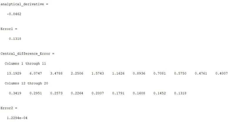

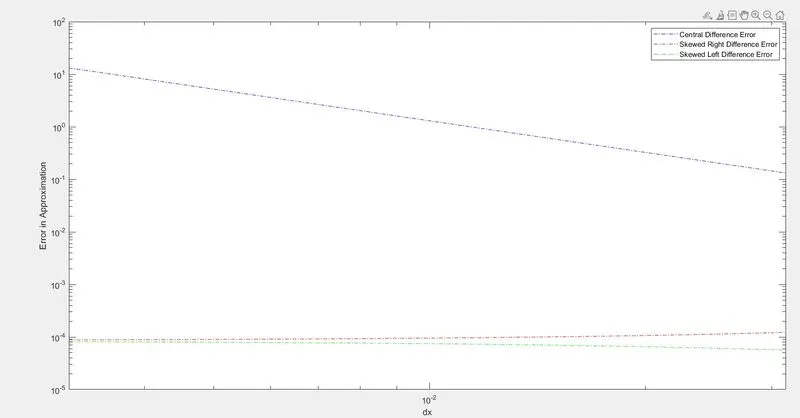
Plot:

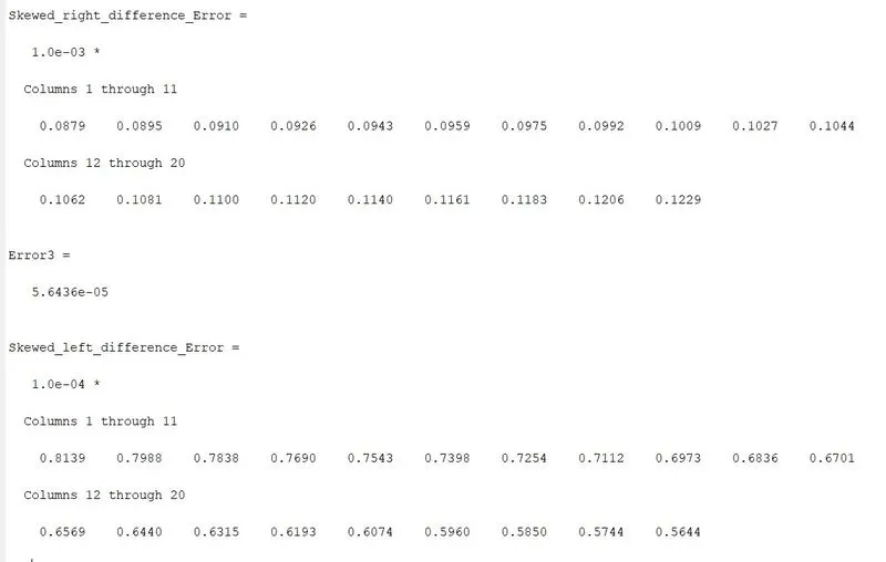
Result:

From the above plot we can inffer that the plot for Skewed left side shows minimum errod as compared to that of central and skewed right difference. The smallest errors are due to the numerical roundoff of constants. In common case we could only have the solution to points of either on positive axix or in the negative axis so we would have to choose either Skewed Left/Right difference for computation and this is why these two methods are better than central diffrence in majority of the cases.