Week 4.1 - Genetic Algorithm
Aim - To optimize the given function and find the global maxima of the same.
Theory - Genetic Algorithms(GA) use biologically inspired operators such as mutation, crossover, and selection & are usually used to generate high-quality solutions to optimization problems.
Phases of GA-
- Initializing the Population - Population Initialization is the first step in the Genetic Algorithm Process. The population is a subset of solutions in the current generation. Population P can also be defined as a set of chromosomes. The initial population is generated randomly using random numbers, which affects the convergence speed and the quality of final solutions.
- Fitness Function - it is the function that we have to optimize, this process is carried out with the help of a number of generations that have been already defined, these values are then used for the reproduction of children.
- Selection - this process involves the selection of the fittest individuals from the population who can pass their genes to the next generations. This process gets inspiration from survival of the fittest, it has to be optimally monitored. The main aim is to identify regions of best solutions.
- Reproduction - The reproduction of offspring is the most important part and mainly occurs in two types :
Crossover - in this process more than one parent is selected and one or more offspring is produced using the genetic material of the parents, in a crossover process is applied usually to higher probability GA.
Mutation - if the probability is very high, the GA gets reduced to a random search, moreover, mutation relates to the exploration of the search space. The mutation is also essential to the convergence of the GA.
The steps involved in GA are:
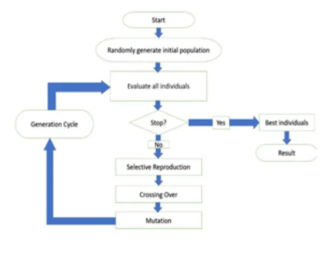
GA is an inbuilt function in Matlab the syntax for the same is as explained below :
x = ga(fun,nvars,A,b,Aeq,beq,lb,ub)
x = ga(fun,nvars,A,b,Aeq,beq,lb,ub,nonlcon)
x = ga(fun,nvars,A,b,Aeq,beq,lb,ub,nonlcon,options)
x = ga(fun,nvars,A,b,[],[],lb,ub,nonlcon,IntCon)
x = ga(fun,nvars,A,b,[],[],lb,ub,nonlcon,IntCon,options)
[x,fval,exitflag,output] = ga(___)
[x,fval,exitflag,output,population,scores] = ga(___)
Description of the syntax :
x = ga(fun,nvars)x, to the objective function, fun. nvars is the dimension (number of design variables) of function.
x = ga(fun,nvars,A,b,Aeq,beq,lb,ub,nonlcon)nonlcon. The function nonlcon accepts x and returns vectors C and Ceq, representing the nonlinear inequalities and equalities respectively. ga minimizes the fun such that C(x) ≤ 0 and Ceq(x) = 0. (Set lb=[] and ub=[] if no bounds exist.)
x = ga(fun,nvars,A,b,Aeq,beq,lb,ub,nonlcon,intcon)x = ga(fun,nvars,A,b,Aeq,beq,lb,ub,nonlcon,intcon,options)intcon take integer values.
We optimize the given function using three case studies and taking the number of iterations as 50(num_iterations=50):
Syntax Explanation of the code:
linspace(x,y,n) - creates an array of x & y values divided in 'n' number of values.
tic - start the stopwatch timer
toc - stop the stopwatch timer
subplot( m, n, p ) - divides the current figure into an m -by- n grid and creates axes in the position specified by p
plot3 - plots the coordinates in a 3d space
shading interp - shading interp varies the color in each line segment and face by interpolating the colormap index or true color value across the line or face.
The program for GA is as shown below :
Function -
% Creating the stalagmite function

function [F]= stalagmite(input)
x=input(1);
y=input(2);
F1 = [sin(5.1*pi*x+0.5)]^6;
F2 = [sin(5.1*pi*y+0.5)]^6;
F3 = exp(-4*log(2)*((x-0.667)^2/0.64));
F4 = exp(-4*log(2)*((y-0.667)^2/0.64));
F  = -(F1*F2*F3*F4) % we use the negative sign to find the global maxima of the function.
GA Program -
% Optimization Code
clc
clear all
close all

% defining our workspace
x=linspace(0,0.6,150);
y=linspace(0,0.6,150);
[xx,yy]=meshgrid(x,y); % creates a 2d mesh array of x & y values
n=50; % number of iterations have been set to 50

for i= 1:length(xx)
for j= 1:length(yy)
    input(1)= xx(i,j);
    input(2)= yy(i,j);
    f(i,j)= stalagmite(input);
end
end

% for unbounded inputs
tic
for i = 1:n
    [res,fopt(i)]=ga(@stalagmite,2);
    xopt(i)=res(1);
    yopt(i)=res(2);
end
study_time1=toc;
figure(1)
subplot(2,1,1)
surf(xx,yy,-f) %generating the surface
shading interp
title 'Statistical Behaviour With Unbounded inputs'
hold on
plot3(xopt,yopt,-fopt,'Marker','o')
subplot(2,1,2)
plot(-fopt)
xlabel('Iterations')
ylabel('F(Max)')

% for bounded inputs
tic
for i = 1:n
    [res,fopt(i)]=ga(@stalagmite,2,[],[],[],[],[0;0],[0.6;0.6]);
    xopt(i)=res(1);
    yopt(i)=res(2);
end
study_time2=toc;
figure(2)
subplot(2,1,1)
surf(xx,yy,-f)
title 'Statistical Behaviour With Bounded inputs'
shading interp
hold on
plot3(xopt,yopt,-fopt,'Marker','o')
subplot(2,1,2)
plot(-fopt)
xlabel('Iterations')
ylabel('F(Max)')

% increasing the number of iterations
tic
options=optimoptions('ga');
options=optimoptions(options,'PopulationSize',250);
for i=1:n
    [res,fopt(i)]=ga(@stalagmite,2,[],[],[],[],[0 0],[0.6 0.6],[],[],options);
    xopt(i)=res(1);
    yopt(i)=res(2);
end
study_time3=toc;
figure(3)
subplot(2,1,1)
surf(xx,yy,-f)
shading interp
title 'Statistical Behaviour with increased no of iterations'
hold on
plot3(xopt,yopt,-fopt,'marker','o')
subplot(2,1,2)
plot(-fopt)
xlabel ('Iterations')
ylabel ('F(Max)')
Results & Case wise Explanation
Case1- Unbounded Values
In the first case, we use unbounded values. The syntax used in the program is explained below :
we have used [x,fval]= ga(fun,nvars)
Where
fun= function
nvars = number of variables
Graph :
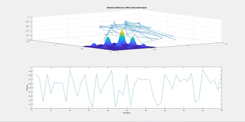
As it can be seen from the graph the unbounded values fail to determine the maxima and fall from the stalagmite graph. In this case, the optimum value is calculated every time the code runs thus not giving accurate results.
The runtime observed was - 38.97sec
Case2- Bounded Values
In the second case, we use bounded values. The syntax used in the program is explained below :
x = ga(fun,nvars,A,b,Aeq,beq,lb,ub)x, so that a solution is found in the range lb ≤ x ≤ ub. (Set Aeq=[] and beq=[] if no linear equalities exist.
Graph :
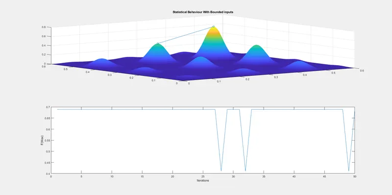
As can be seen from the graph by providing the lower and upper bound we observe the randomness of values has been greatly reduced.
The runtime observed was - 24.8431sec
Case3- Increasing the number of iterations
We increase the number of iterations or the population size from 50 to 250.
The syntax used for this is
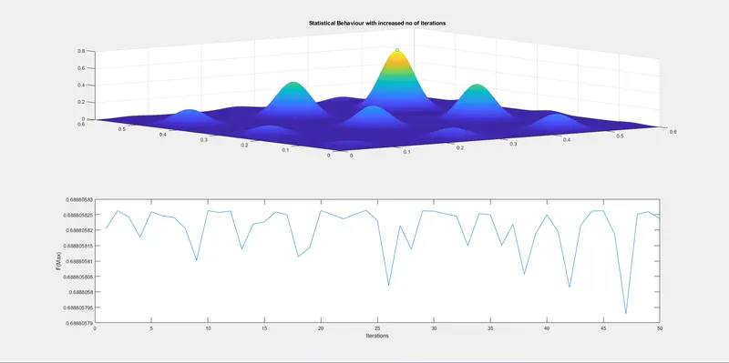
The runtime observed was - 130.81sec, clearly, the run time is maximum in this case but convergence is better and we can find the global maxima.
Result: The optimization code has been successfully run and different GA methods have been understood.