Week 3 - Solving second order ODEs

Objective - To create a Matlab program that simulates the motion of a pendulum.

Theory- The motion of a simple pendulum is given by the governing equation :

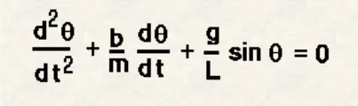
To solve the above differential equation we need to bring the 2nd order terms into 1st order and write the equation in matrix form for Matlab to solve it, the following procedure is used:

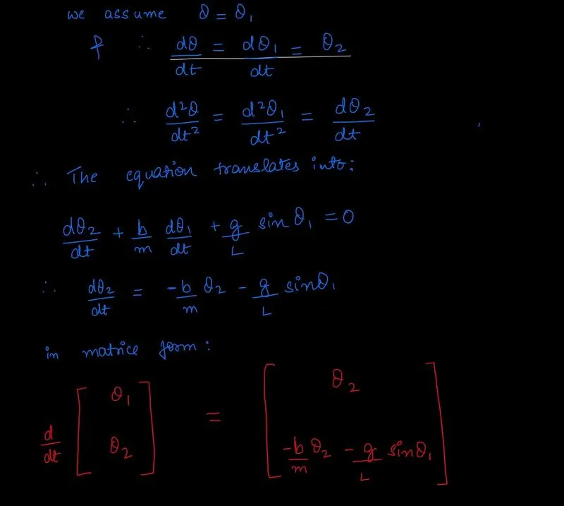
After getting the matrice form of the equation we create a function for the same which we can recall in the original program, this function is dependent on (t, theta, b,g,l,m) :

FUNCTION SCRIPT:

% The function is dependent on time, theta , b, gravitational force, length
% & mass :
function [dtheta_dt]= ode_func(t,theta,b,g,l,m) 

theta1=theta(1);
theta2=theta(2);

dtheta1_dt=theta2; % as assumed
dtheta2_dt= -(b/m)*theta2-(g/l)*sin(theta1); % as solved for
dtheta_dt=[dtheta1_dt;dtheta2_dt]; % matrice form 
end

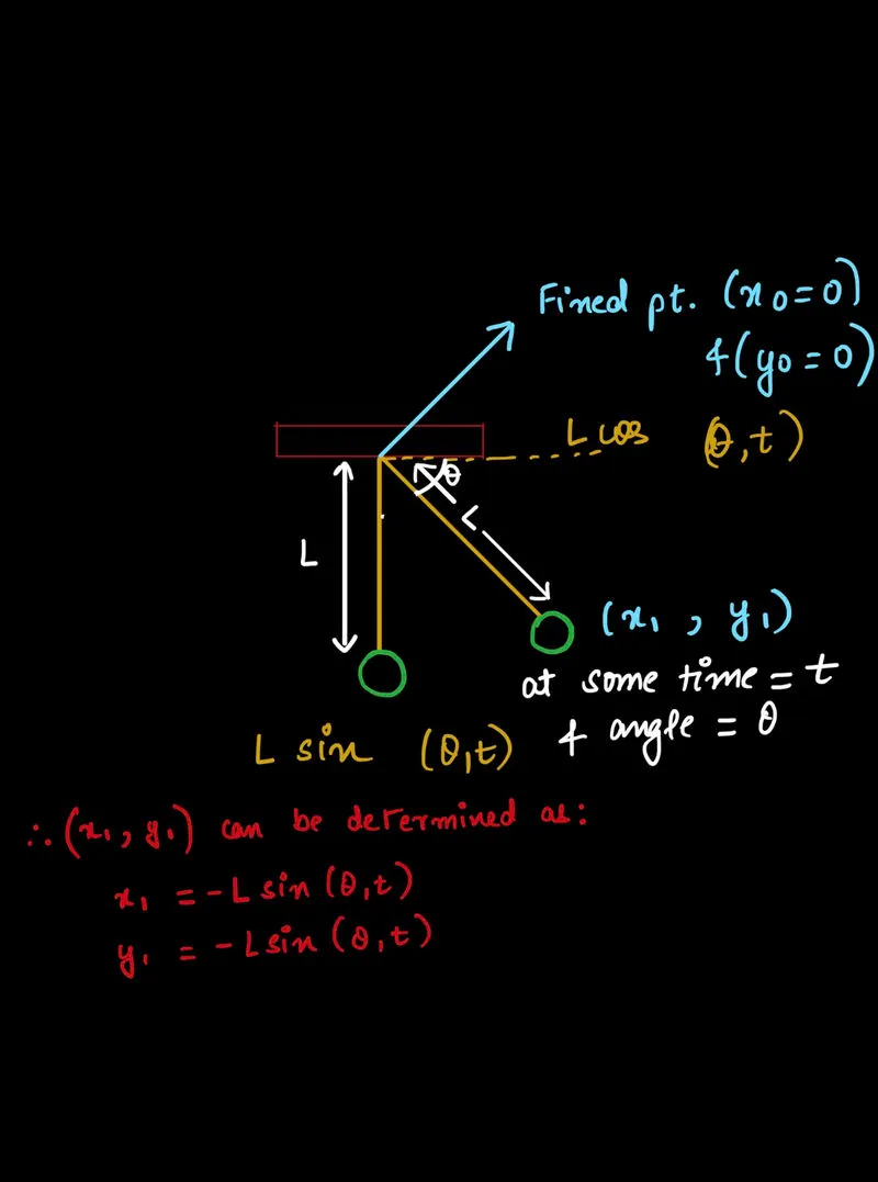
For animating the problem we also need to understand how the position of the pendulum changes, the position variation is as shown below :

Main Code for Simple Pendulum :

Explanation of Syntax used in the code :

ode45 -- solves ordinary differential equations in Matlab — medium order method

legend -- creates a dialogue box explaining the parameters of the figure.

marker indices -- defines the position of the placement of the marker, the position of the marker has been found out by idmax=find(theta_0==max(theta_0))

Suitable Explanations have been given in the code in the form of comments :

clc 
close all
clear all

% Inputs - damping coefficient, gravitational force, length & mass.
b=0.05;
g=9.81;
l=1;
m=1;

theta_0=[0;3]; % values of theta 
t_span=linspace(0,20,500); % time span ranging from 0-20 with 500 values on between.

[t,results]= ode45(@(t,theta) ode_func(t,theta,b,g,l,m),t_span,theta_0); % solves the ordinary differential equation which is a function of t,theta

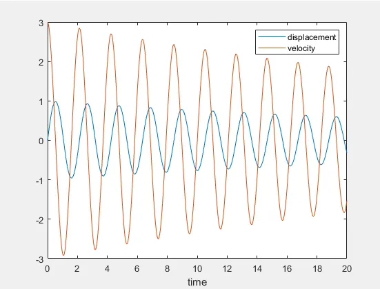
plot(t,results(:,1)) % plots the graph on how results vary with time.
hold on % lets the other graphs be accomodated in one.
plot(t,results(:,2)) % plots the graph on how results vary with time.
xlabel 'time'
legend ('displacement','velocity',Location='northeast') % (creates a dialogue for graph parameters)

% to make the animation work we create a for loop .
for i=1:length(t) 
    x1=-l*sin(results(i,1)); % x-position of pendulum at time t
    y1=-l*cos(results(i,1)); % y-position of pendulum at time t
    figure(2)
    x0=0; % inital x-position of pendulum at time t=0.
    y0=0; % inital y-position of pendulum at time t=0.
    idmax=find(theta_0==max(theta_0)); %to find the end of the pendulum where marker has to be created.

    % plotting and creating marker "o" so that it looks like a pendulum.
    plot([x0 x1], [y0 y1],LineWidth=4,Marker="o",MarkerIndices=idmax,MarkerEdgeColor='r',MarkerFaceColor='b',MarkerSize=20)
    axis ([-1 1 -2 0]) % sets the limits of the axis.
    legend ('motion of a simple pendulum',Location='northeast') % (creates a dialogue for graph parameters)
    pause(0.03); % sets the time interval between figures.
    N(i)=getframe(gcf); % collects the frame from the current figure handle.
end

 movie(N) % creates a movie of the frames collected
 myvideo=VideoWriter("Pendulum.avi",'Uncompressed AVI'); % saves the movie in the format desired.
 open(myvideo) % opens the videofile.
 writeVideo(myvideo,N); % saves the videofile to the current folder.
 close(myvideo); %closes the videofile.

The graph between Displacement, Velocity & Time :

Youtube link for the animation of the pendulum :

https://youtu.be/7fbmng2c6bI

Result:

The Matlab program to obtain the motion of the pendulum has been successfully created.