Assignment 4-RADIOSS Material Laws Challenge

Objective - To run crash analysis on the given model using different material laws in Radioss and compare the results in different cases.

Procedure :

Case 1 :

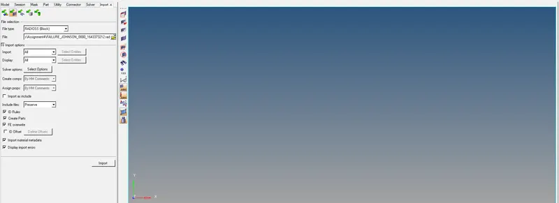
Open hyper mesh and import the model as shown :

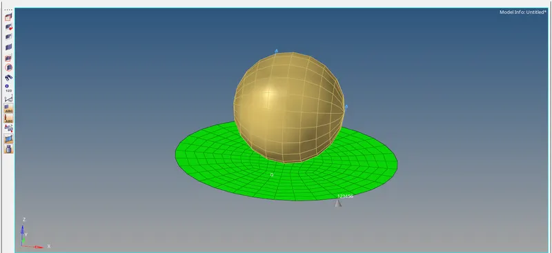
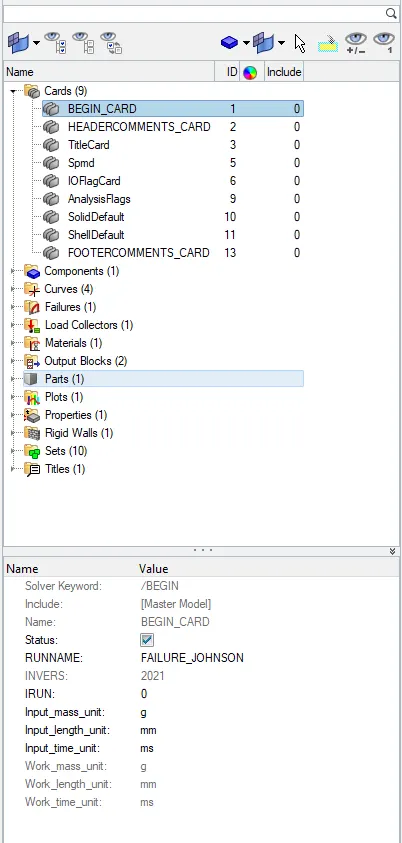
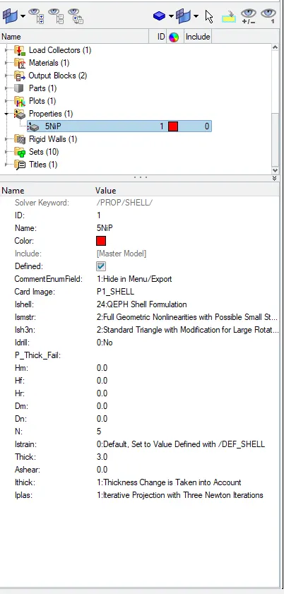
In the first case, we run the simulation without changing any values. The default set up is as shown below :

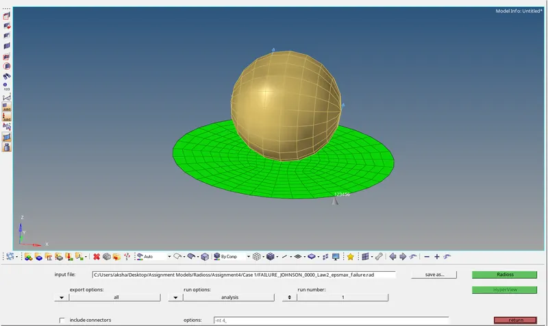
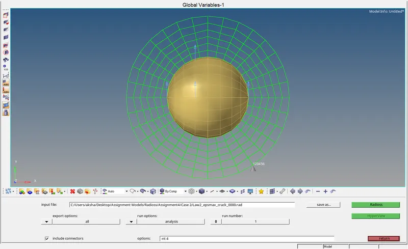
To run the analysis we go to the analysis>>Radioss, then we give the file name, and we give the -nt4 as an option so that it utilizes 4 cores of the CPU and performs the simulation faster.

Finally, we click on Radioss to run the simulation:

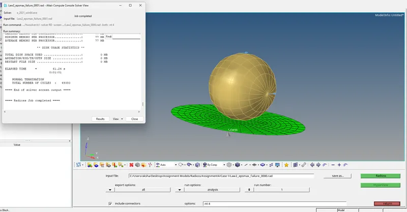
The solver runs and shows the ongoing tasks, and we can also access the files from the solver.

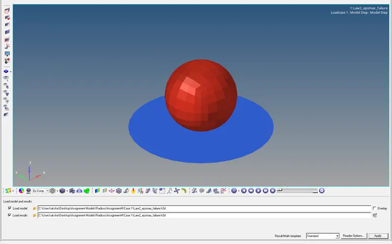
After the job completion we switch to the hyperview utility to visualize the results as shown below:

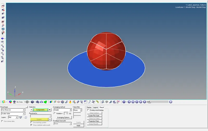
We switch on the elements and give the 'von mises' contour with the averaging method as 'Simple' :

Contour Plot:

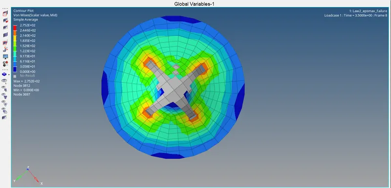
The maximum stress is seen to be 275MPA.

The simulation of the 1st case is shown in the video.

Next, we check the energy and the mass error as shown below :

We can access the errors in the. out file saved in the folder:

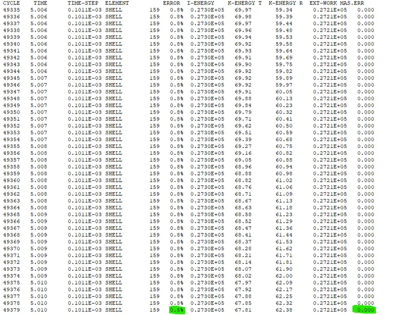
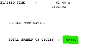
The energy error is 0.8% and the mass error is 0, both are in the acceptable ranges.

The simulation was completed in 62.40s and the total number of cycles is 49380.

Now we plot the energies for the analysis as shown below:

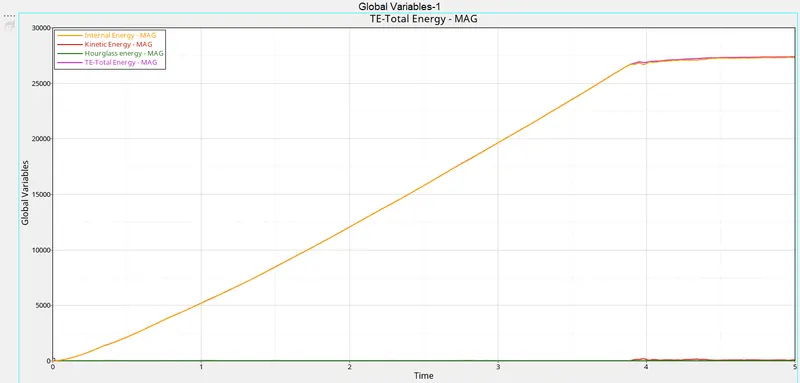
In the above graph, we can see that the hourglass energy is zero, and the Internal energy of the system increases with time due to the forces acting on the elements.

Case 2:

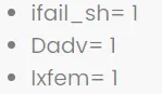
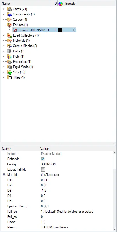
In this case, we change the values in the Failure card as follows:

Now we run the simulation and repeat the steps performed above:

Contour Plot:

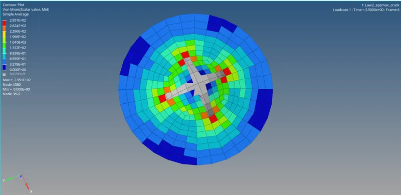
Crack can be seen in the simulation since the Ixfem = 1 & Ifail=1 which allows the elements to crack and not be deleted.

The maximum stress is 295.1 MPA which is higher than in the previous case.

Energy Graph:

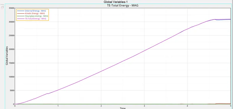
The internal energy and total energy increase with time and flatten after 3ms.

Next, we check the energy and the mass error as shown below :

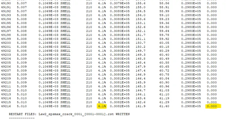
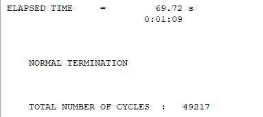
The energy error is 4.1% and the mass error is 0, both are in the acceptable range, the total cycles are 49217 and the elapsed time is greater than the previous case at 69.72 sec.

Case 3:

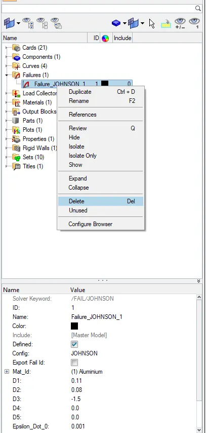
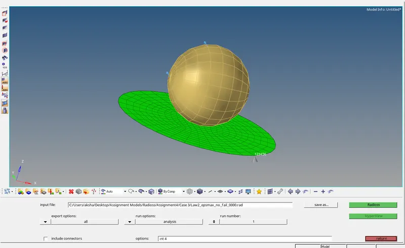
We delete the failure card from the model and then run the simulation as shown below :

Contour Plot:

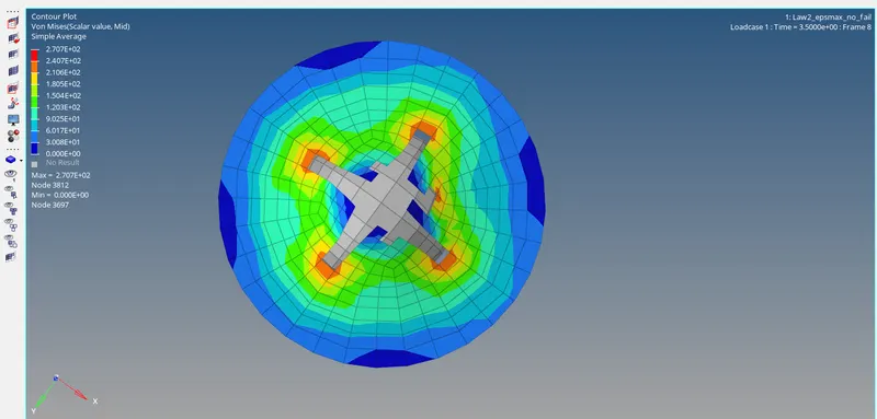
There is no crack observed because of the deletion of the failure card. The elements can be seen as being deleted in the simulation.

The maximum stress observed is 270.7MPA.

Energy Graph:

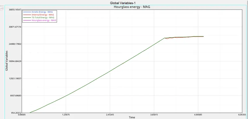
The hourglass energy is zero, the internal energy increases with time as seen in previous cases.

We check for the energy and mass errors in the output file:

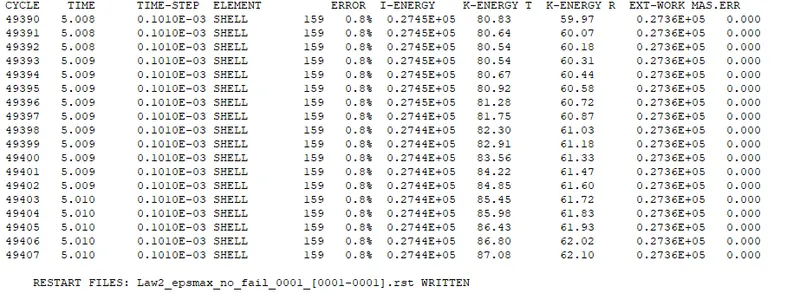
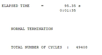
The energy error is 0.8% which is in the acceptable range and the mass error is 0.

The elapsed time is 95.35sec and the total no of cycles is 49408.

Case 4:

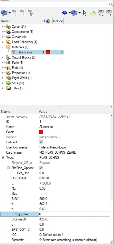
In this case, we run the simulation with Eps_P_Max = 0 as shown below:

We run the simulation and the contour plot is shown below:

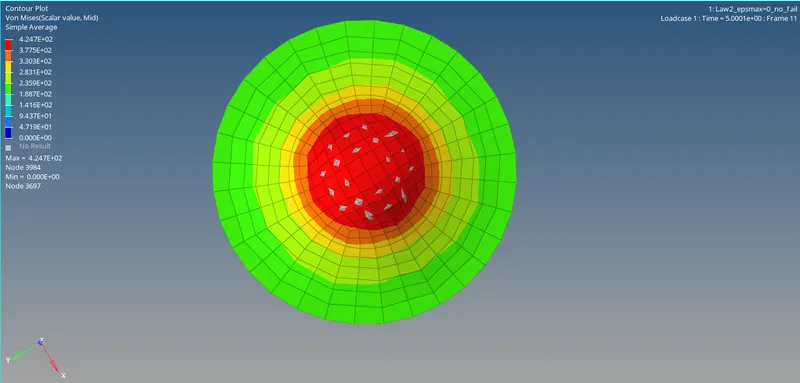
In the simulation, we observe that the elements do not fail as there is no failure criterion applied.

The maximum stress value is observed to be 424.7MPA as the sigma_max has been set to 425MPA.

Energy Graph:

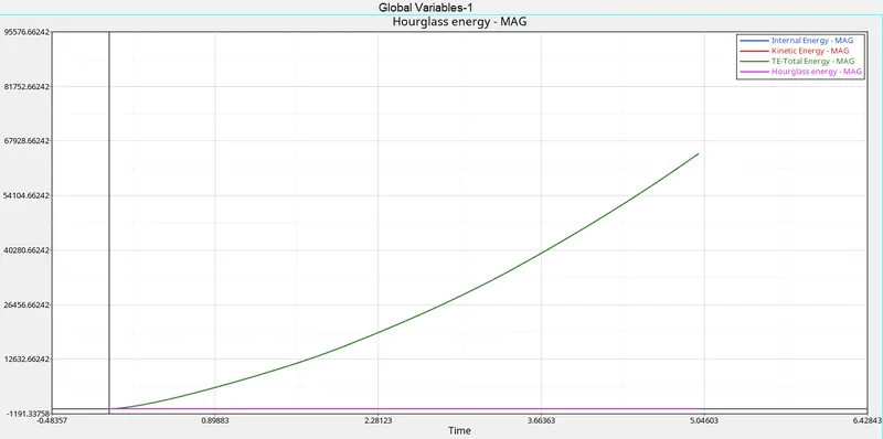
No hourglass energy is developed in the simulation and the internal energy is equal to the total energy of the system.

Now we check for the energy and mass errors:

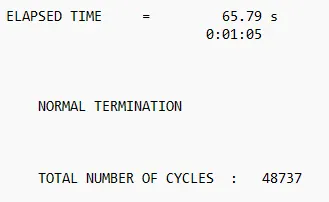
The energy error is 3% which is in the acceptable range and the mass error is 0.

The elapsed time is 65.79sec and the total no of cycles is 48737, the time taken for the simulation is less than the other three simulations.

Case 5:

Changing law 2 (Elastoplastic material) to law 1(linear elastic material)with the same values of E (youngs modulus), density, and Poisson's ratio.

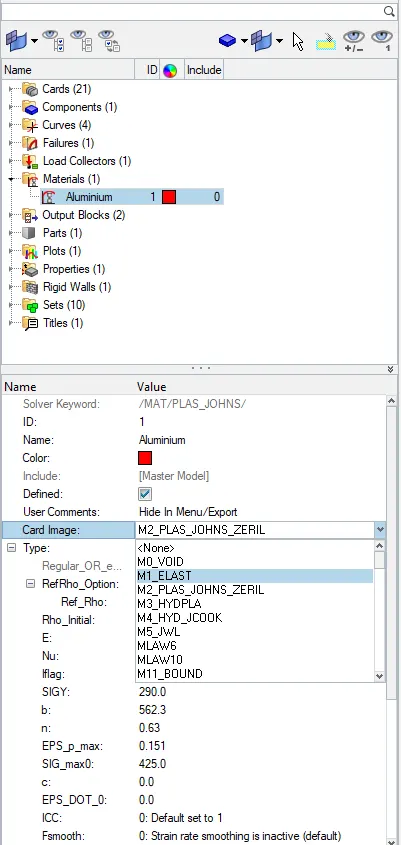
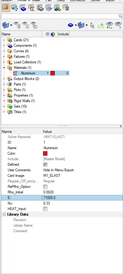
Now we run the simulation and the contour plot for the same is shown below:

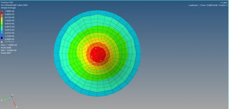
No failure of elements is observed in this case due to linear elastic material, there is no plastic region in the material hence no elements fail and no plastic strain is observed in the simulation.

Energy Graph:

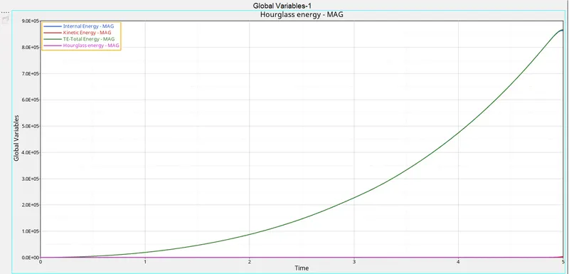
The internal energy and total energy intercept each other and the hourglass energy is zero.

Now we check for the energy and mass errors:

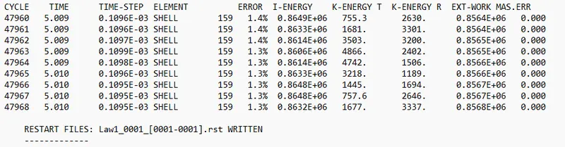
The energy error is 1.3% which is in the acceptable range and the mass error is 0.

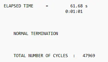
The total time taken for the simulation is 61.68sec and the no of cycles is 47969.

Case6:

In this case, we use Material Law 36 which is for isotropic elastoplastic materials.

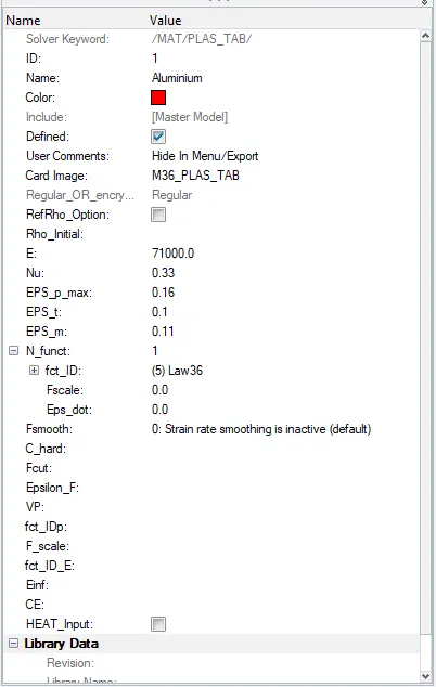
The material card for the given case is as shown:

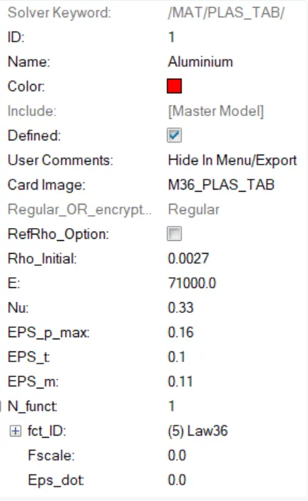
Now we create a user-defined curve as shown below:

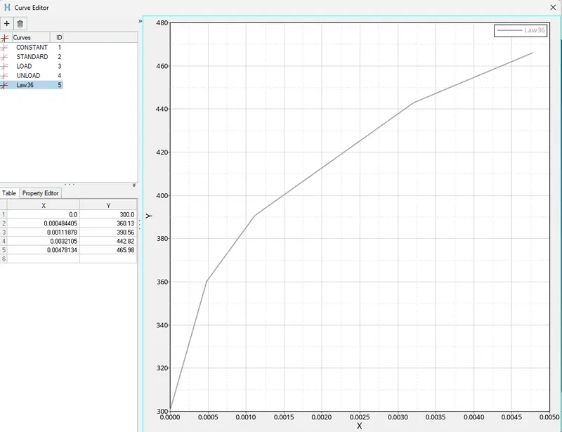
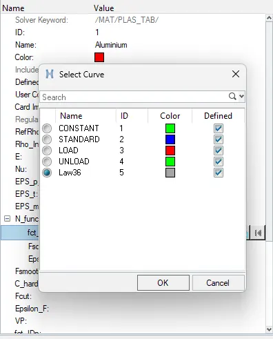
The material card is now made as per the specifications shown below:

Now we run the simulation and the contour plot for the same is shown below:

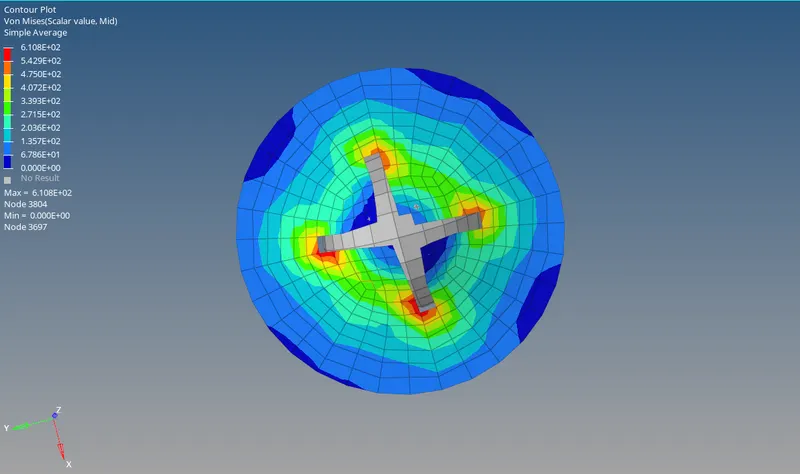
The maximum stress observed is 610.8 MPA. Once the EPS_p (plastic strain) reaches EPS_p_max, in one integration point, the elements are deleted as seen in the simulation.

Energy Graph:

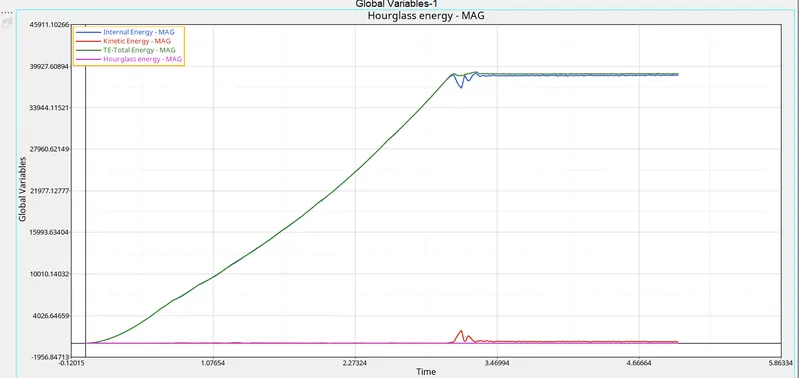
There is an almost linear relation between internal energy and time till past the 3.8ms mark where many elements get deleted at once. When the elements are deleted, the energy from each element is released, resulting in the plateauing of the curve.

We check for energy and mass errors in the output file:

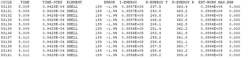
The energy error is -1.9% which is in the acceptable range and the mass error is 0.

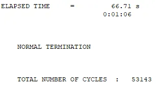
The total time taken for the simulation is 66.71sec and the no of cycles is 53143.

Case 7:

Changing the material card to Law 27, this law combines johnson cook material with the brittle failure method.

We import the law_27 file & change the recommended properties for shell elements and proceed as shown below:

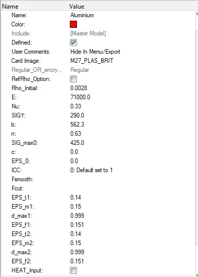
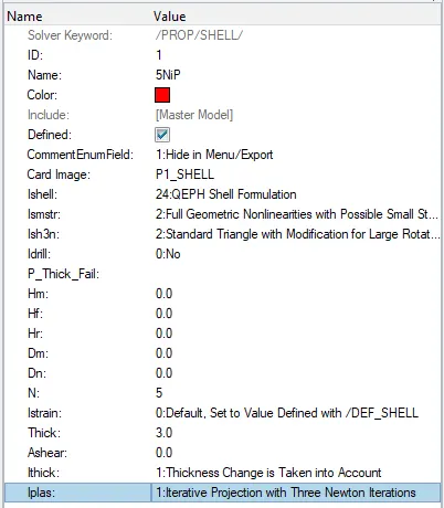
The simulation has been run and the contour plot is as follows:

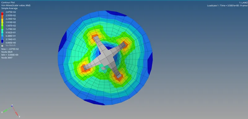
The maximum stress developed in the simulation is 287.5 MPa, which is below the Plasticity yield stress value of 290 MPa.

The material can be seen breaking after the crack propagated to the boundary of the material.

Energy Graph:

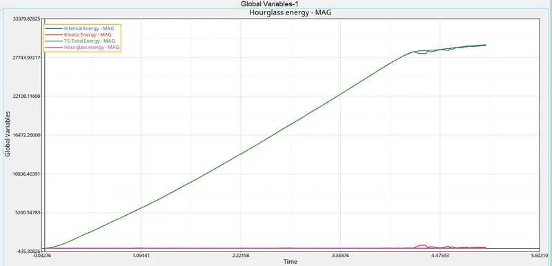
There is no hourglass energy present in the model, the internal energy and total energy can be seen to increase with time.

Now we check the energy & mass errors:

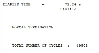
The energy error is 0.8% and the mass error is zero.

The total simulation time is 72.24 sec & the total no of cycles is 49508.

Results:

CASE	Material Law Used	Material Law Description	Energy Error	Mass Error	Simulation Time	No of cycles	Max. Stress Observed	Element Behaviour Observed
1	Law 2	Johnson-Cook model	0.8%	0	62.40	49380	275 MPA	Deleted
2	Law 2	Johnson-Cook model with failure plastic strain (EPS_p_max) and fail_Johson card enabled.	4.1%	0	69.72	49217	295.1 MPA	Deleted after crack formation.
3	Law 2	Johnson-Cook model with the removal of the failure card.	0.8%	0	95.35	49408	270.7MPA	Deleted
4	Law 2	Johnson-Cook model with the removal of both the failure plastic strain (EPS_p_max) and the fail_Jhonson failure card.	3%	0	65.79	48737	424.7MPA	Can not be deleted due to a lack of properties.
5	Law 1	Linear elastic material	1.3%	0	61.68 sec	47969	10890 MPA	Preserved
6	Law 36	Elasto-plastic material	-1.9%	0	66.71 sec	53143	610.8 MPA	Deleted
7	Law 27	Brittle failure model	0.8%	0	72.24 sec	49508	287.5 MPa	Deleted

Case 2 is found to be the most practical choice as In Case 2 we used Ifail_sh, Dadv, and Ixfem as part of the Fail/JOHNSON card.

Ixfem = 1, means the elements will crack and fail. With the use of Dadv, crack propagation can also be seen here, with elements being deleted only when the crack reaches them.

Conclusion:

All the different cases have been compared and Case 2 has been found to be the closest to the practical scenario.