Week - 2 - Explicit and Implicit Analysis
Objective- to establish a clear difference b/w implicit and explicit analysis and to solve an example of the same by both approaches.
Procedure-
1. Difference b/w Implicit and explicit analysis :
|
S.No. |
Implicit | Explicit |
| 1 | Used for small deformations. | Used for larger deformations in lesser time. |
| 2 | We find displacement by the inversion of the stiffness matrix. [K] | We find acceleration by the inversion of the mass matrix. [M] |
| 3 |
For Each Increment: Stiffness Matrix Updated. Next increment of load defined. Newton Raphson- to enforce equilibrium. |
For Each Increment: Stiffness Matrix Updated. Next increment of load defined. Direct solution. |
| 4 | the implicit scheme is unconditionally stable, i.e. for any initial assumption of (deltaT) the solution converges. |
the explicit scheme is conditionally stable, i.e. it has to satisfy the critical time step to be conditionally stable. i.e. - `triangletletriangletcr` `triangletcr=L/c` `c=(E/c)^0.5` |
| 5 | accuracy is higher | accuracy is lower |
| 6 | Extremely time consuming for larger models | Computationally efficient for larger models with relatively short dynamic response times. |
| 7 | no mathematical time limit for a solution | depends on wave propagation speed & characteristic length of the element. |
| 8 | cost is higher | cost is lower |
| 9 | used when the effect of strain rate is lower | used when strain rates have a significant effect. |
| 10 | can solve moderate contact conditions | can solve most complex contact conditions |
2. Explicit Analysis:
Step 1 -
K=`3*u^2+18*u+4`; K(u°)=4
`triangleU`=`triangleF`/K ; `triangleU`= 0.25 ;
u1 = u° + `triangle`u1 = 0 + 0.25 = 0.25; Fint = 1.578; Residual = 1.578-1 = 0.578
Step 2 -
K=`3*u^2+18*u+4`; K(u⊃1;)= 8.6875
`triangleU`=`triangleF`/K ; `triangleU`= 0.1151 ;
u2 = u1 + `triangle`u2 = 0.365108; Fint = 2.708 ; Residual = 2.708-2 = 0.708
Step 3 -
K=`3*u^2+18*u+4`; K(u⊃2;)= 10.9718
`triangleU`=`triangleF`/K ; `triangleU`= 0.091142 ;
u3 = u2 + `triangle`u3 = 0.45625; Fint = 3.7934; Residual = 3.7934-3 = 0.7934.
|
Step ∆i |
∆Fi |
∆ui |
Ui |
(Fext)i |
(Fint)i |
Residual (fint-Fext) |
|
1 |
1 |
0.25 |
0.25 |
1 |
1.578 |
0.578 |
|
2 |
1 |
0.1151 |
0.3651 |
2 |
2.708 |
0.708 |
|
3 |
1 |
0.09114 |
0.45625 |
3 |
3.7934 |
0.7934 |
3. Implicit Analysis:
For Implicit analysis we follow the procedure as follows:
The correction term is:
`deltau=-[K(u)]^-1 * R`
Step1:
Using u=0, we get the following values (Refer to Spreadsheet for calculation):
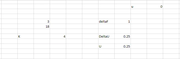
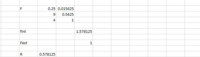
Since R > 10^-2
Newton Raphson iterations are necessary to enforce equilibrium:
We calculate the correction = -0.06655
Corrected u (1) = u1 + corr = 0.25 + (-0.06655) = 0.18345
Fint=1.042859; Residual = 0.042859 < 10>
One more newton Raphson iteration is necessary:
Calculating the correction (Delta u2) = delta u1 + delta u2 = -0.06655 – 0.00571 = -0.07226
Now, u2 = 0.25 - 0.072226 = 0.17774
Fint (0.17774) = 1.000899
Residual = 0.000899 < 10>
Thus no further iterations are required.
Step 2:
U (2) = u2 + corr = 0.365108 + (-0.06453) = 0.300578
Fint=2.042593; Residual = 0.042593 < 10>
One more newton Raphson iteration is necessary:
Calculating the correction (corr1+corr2) = -0.06453-0.0044 = -0.06893
Now, u2 = 0.365108 + (-0.06893) = 0.296178
Fint (0.296178) =2.000186
Residual = 0.000186 < 10>
Thus no further iterations are required.
Step 3:
U (3) = u3 + corr = 0.45625 + (-0.06181) = 0.3944
Fint=3.038912; Residual = 0.038912 < 10>
One more newton Raphson iteration is necessary:
Calculating the correction (corr1+corr2) = -0.06181-0.00336 = -0.06517
Now, u2 = 0.45625 + (-0.06517) = 0.39108
Fint (0.296178) =3.000625
Residual = 0.000625 < 10>
Thus no further iterations are required.
Exact vs explicit vs implicit :
| F=1 | F=2 | F=3 | |
| Exact | 0.17762 | 0.29616 | 0.39103 |
| 0.25 | 0.3651 | 0.45625 | |
| 0.17774 | 0.296178 | 0.39108 |
The plot is as shown:
Result - The explicit and implicit analysis has been carried out successfully.