Week 3 - Solving second order ODEs
Aim:
To write a code for Simple Pendulum with help of ordinary differential equation in the format of python using Sublime.
Theory:
A pendulum is a body suspended from a fixed support so that it swings freely back and forth under the influence of gravity. When a pendulum is displaced sideways from its resting, equilibrium position, it is subject to a restoring force due to gravity that will accelerate it back toward the equilibrium position. When released, the restoring force acting on the pendulum's mass causes it to oscillate about the equilibrium position, swinging it back and forth.
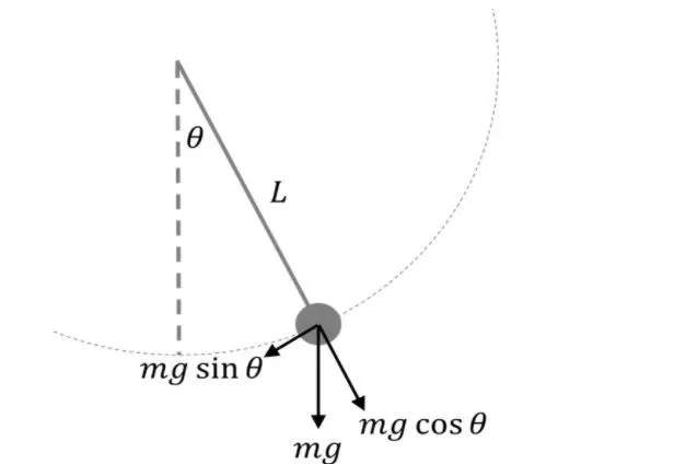
Derive the equation for a simple pendulum, By applying Newton's secont law for rotational systems, the equation of motion for the pendulum may be obtained
Cancelling mass on each side and writing in standard form gives:
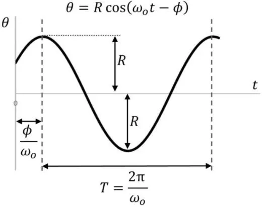
When the angle θ is small, perhaps less than 15 deg, then sinθ≈θ. This is referred to as the small angle approximation. This greatly simplifies the differential equation:
θ''+(b/m)θ'+(g/L) =0
import numpy as np
from scipy.integrate import odeint
import matplotlib.pyplot as plt
import math#write the function for the ordinary equation
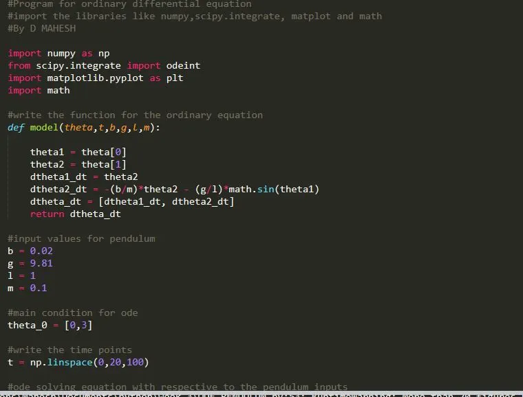
def model(theta,t,b,g,l,m):
theta1 = theta[0]
theta2 = theta[1]
dtheta1_dt = theta2
dtheta2_dt = -(b/m)*theta2 - (g/l)*math.sin(theta1)
dtheta_dt = [dtheta1_dt, dtheta2_dt]
return dtheta_dt#input values for pendulum
b = 0.02
g = 9.81
l = 1
m = 0.1
#main condition for ode
theta_0 = [0,3]
#write the time points
t = np.linspace(0,20,100)3. Now write the input values of simple pendulum and define theta in the form of array and write the time inputs with help of numpy linespace.
#ode solving equation with respective to the pendulum inputs
theta = odeint(model,theta_0,t,args = (b,g,l,m))
#now plot the results
plt.plot(t,theta[:,0],'b-',label=r'$\frac{d\theta_1}{dt}=\theta2$')
plt.plot(t,theta[:,1],'r--',label=r'$\frac{d\theta2}{dt}=\frac{b}{m}\theta_2-\frac{g}{L}sin\theta_1$')
plt.ylabel('Theta')
plt.xlabel('Time')
plt.grid()
plt.show()
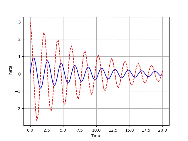
4. Now define theta in the form of ode and plot the graph between theta vs time and save the plot.
#to create a animation for simple pendulum write loop counter
loop_counter = 1
tmp = theta[:,0]
for i in tmp:
x_start = 0
y_start = 0
x_end = 1*math.sin(i)
y_end = -1*math.cos(i)
#plot the animation
plt.figure()
#to plot the string
plt.plot([x_start,x_end],[y_start,y_end],linewidth=3)
#bob of pendulum
plt.plot(x_end,y_end,'o',markersize=24,color='r')
#plot the rigid support
plt.plot([-0.5,0.5],[0,0],linewidth=12,color='k')
#plot the vertical line for reference
plt.plot([0,0],[0,-1.5],'--',color='y')
plt.xlim([-1.25,1.25])
plt.ylim([-2,1])
plt.title('SIMPLE PENDULUM ANIMATION')
filename = 'simplepenanim%01d.png' % loop_counter
plt.savefig(filename)
loop_counter = loop_counter + 15. Nothew create an animation for the simple pendulum in the format of loop counter and here define the starting point of the bob and ending point with the help of 'i tmp' in for loop and to see the string and the bob we need to plot them by defining the markersize and color and save the file.
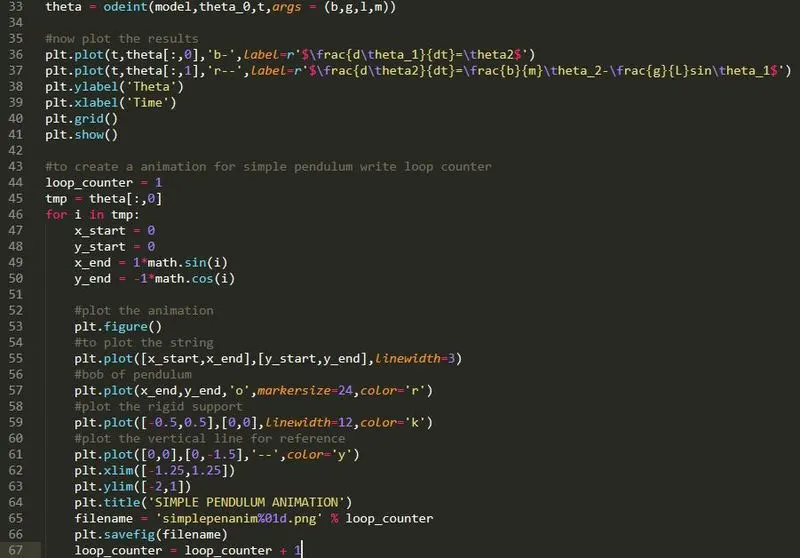
Code and Animation:
#Program for ordinary differential equation
#import the libraries like numpy,scipy.integrate, matplot and math
#By D MAHESH
import numpy as np
from scipy.integrate import odeint
import matplotlib.pyplot as plt
import math
#write the function for the ordinary equation
def model(theta,t,b,g,l,m):

	theta1 = theta[0]
	theta2 = theta[1]
	dtheta1_dt = theta2
	dtheta2_dt = -(b/m)*theta2 - (g/l)*math.sin(theta1)
	dtheta_dt = [dtheta1_dt, dtheta2_dt]
	return dtheta_dt
#input values for pendulum
b = 0.02
g = 9.81
l = 1
m = 0.1

#main condition for ode
theta_0 = [0,3]

#write the time points
t = np.linspace(0,20,100)
#ode solving equation with respective to the pendulum inputs
theta = odeint(model,theta_0,t,args = (b,g,l,m))

#now plot the results
plt.plot(t,theta[:,0],'b-',label=r'$\frac{d\theta_1}{dt}=\theta2$')
plt.plot(t,theta[:,1],'r--',label=r'$\frac{d\theta2}{dt}=\frac{b}{m}\theta_2-\frac{g}{L}sin\theta_1$')
plt.ylabel('Theta')
plt.xlabel('Time')
plt.grid()
plt.show()
#to create a animation for simple pendulum write loop counter
loop_counter = 1
tmp = theta[:,0]
for i in tmp:
	x_start = 0
	y_start = 0
	x_end = 1*math.sin(i)
	y_end = -1*math.cos(i)

	#plot the animation
	plt.figure()
	#to plot the string
	plt.plot([x_start,x_end],[y_start,y_end],linewidth=3)
	#bob of pendulum
	plt.plot(x_end,y_end,'o',markersize=24,color='r')
	#plot the rigid support
	plt.plot([-0.5,0.5],[0,0],linewidth=12,color='k')
	#plot the vertical line for reference
	plt.plot([0,0],[0,-1.5],'--',color='y')
	plt.xlim([-1.25,1.25])
	plt.ylim([-2,1])
	plt.title('SIMPLE PENDULUM ANIMATION')
	filename = 'simplepenanim%01d.png' % loop_counter
	plt.savefig(filename)
loop_counter = loop_counter + 1 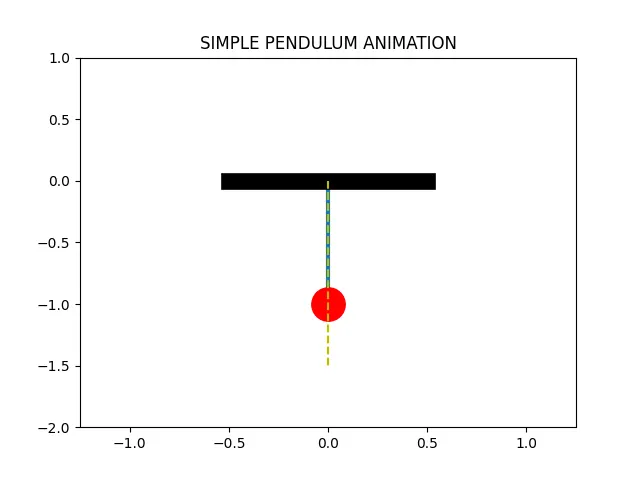
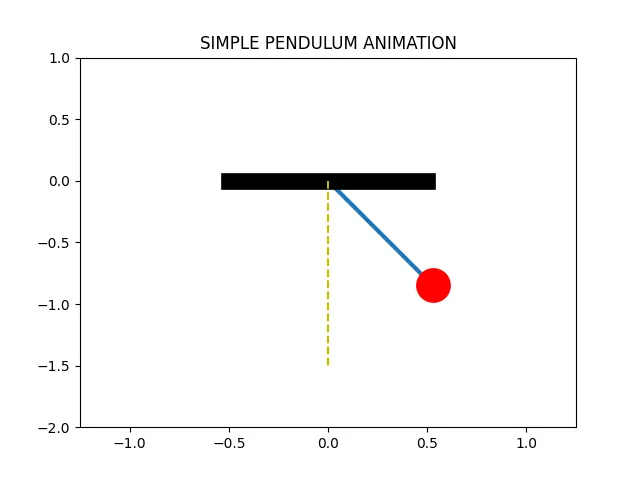
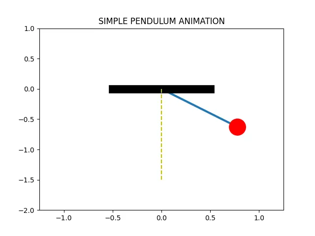
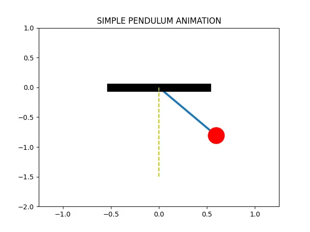
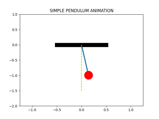
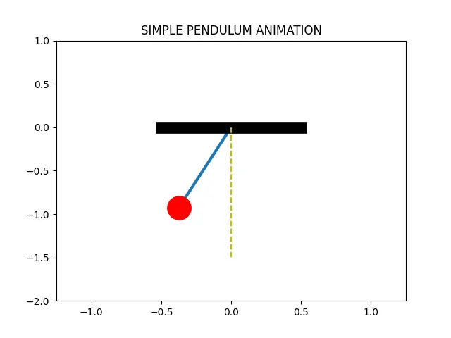
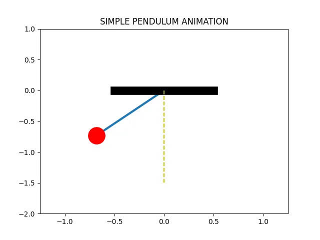
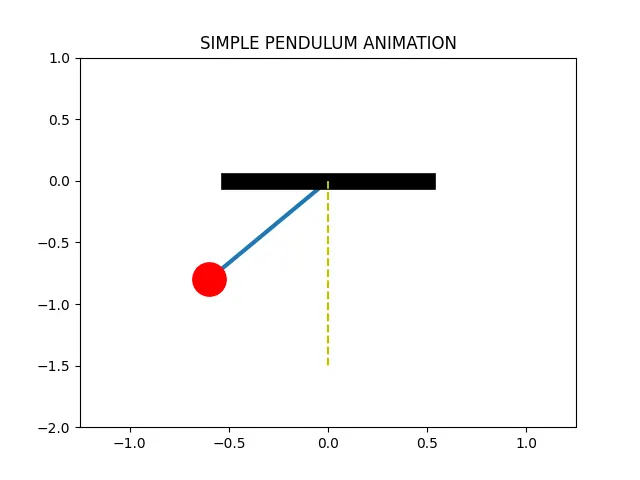
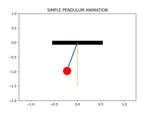
Conclusion:
Thus we written the code for simple pendulum and plot the graph for theta vs time and animated the simple pendulum with the help of python script.