Week - 8 Mass Scaling

Objetive :

To reduce the simulation time of given analysis using the mass scaling method( 8%) and compare this with the both explicit and implicit analysis.

Theory :

What is mass scaling?

Anytime you add nonphysical mass to increase the timestep in a dynamicanalysis, you affect the results (think of F=m*a). Sometimes the effect is insignificant and in those cases adding nonphysical mass is justifiable. Examples of such cases may include the addition of mass to just a few small elements in a noncritical area or quasi-static simulations where the velocity is low and the kinetic energy is very small relative to the peak internal energy. In the end, it's up to the judgement of the analyst to gage the affect of mass scaling. You may have to reduce or eliminate mass scaling in a second run to gage the sensitivity of the results to the amount of mass added.

One can employ mass scaling in a selective manner by artificially increasing material density of the parts you want to mass-scale. This manual form of mass scaling is done independently of the automatic mass scaling invoked with DT2MS in *CONTROL_TIMESTEP.

When DT2MS is input as a negative value, mass is added only to those elements whose timestep would otherwise be less than
|DT2MS|. By adding mass to these elements, their timestep becomes equal to |DT2MS|. An infinite number of combinations of TSSFAC and DT2MS will give the same product, i.e., timestep but the added mass will be different for each of those combinations. The trend is that the bigger |DT2MS| (and the smaller TSSFAC while TSSFAC*|DT2MS|=const), the greater the added mass. In return, stability may improve as TSSFAC is reduced (just as in non-mass-scaled solutions). If stability is a problem with the default TSSFAC of 0.9, try 0.8 or 0.7. If you reduce TSSFAC, you can increase |DT2MS| proportionally so that their product, and hence timestep, is unchanged.

Procedure :

Step 1: Import the given analysis model into the ls-dyna and here we can see that all keycards are specified to the model.

Step 2 : As all key cards are specified we need to perform a simulation and reduce the whole simulation time with the mass scaling. Time step key card is used for the mass scaling.

Step 3 : In order to find out the perfect mass scaling value which is under the 8% we need to do it in trail and error method.

Trail 1: For the first trail we are not using the time step keycard because we need to know how much time consumes for complete simulation.

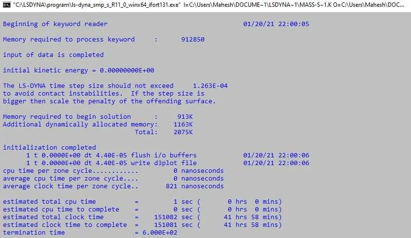
From above we can see that solving time is huge for this simulation, to reduce this we need to find out the exact mass sacling value or dt2ms value.

Trail 2 : For second trail we are going to use the default values time step card and the dt2ms and tssfac values are -3.5E-05 and 0.9.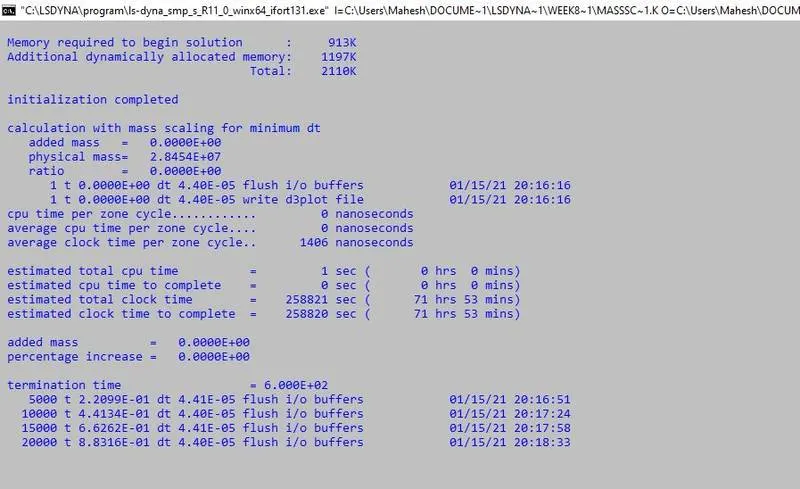

For default value of time step card we are not getting the perfect time so we need to start with the decreasing the dt2ms value to find the perfect mass scaling which is under the 8 percentage.

Trail 3 : From this trail we are not changing any values in the time step card except the dt2ms value, here we are using the dt2ms = -3.0E-05.

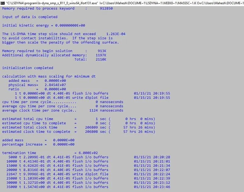
Here are also problem time is huge and we are not getting the percentage increase.

Trail 4 : For this trail dt2ms is -2.5E-05.

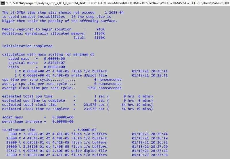
Trail 5 : For this trail dt2ms is -2.0E-05.

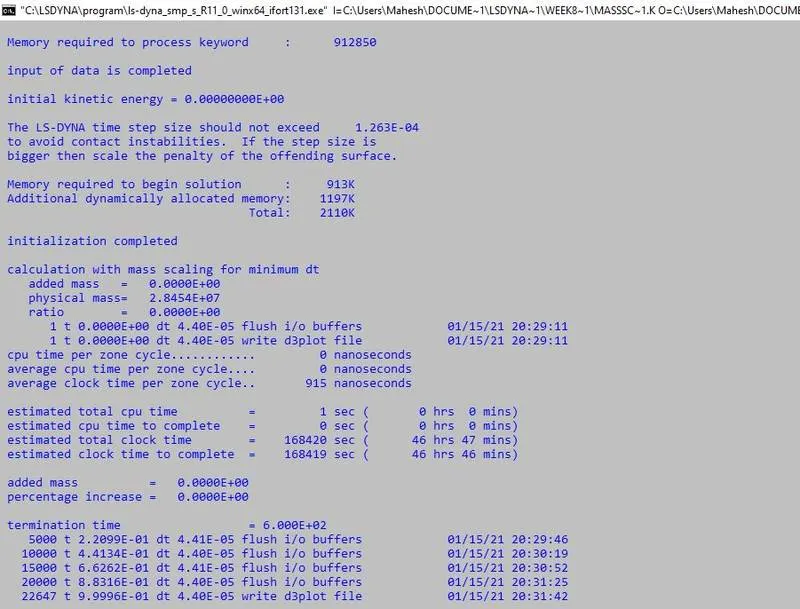
Trail 6 : For this trail dt2ms value is -1.5E-05

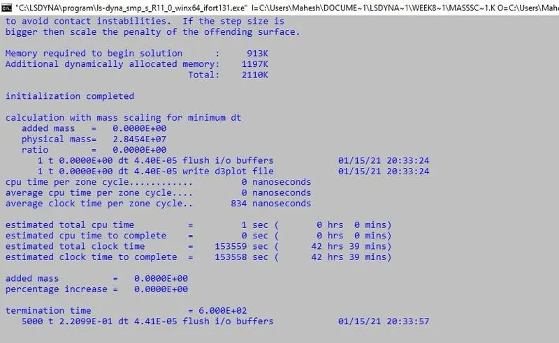
Here we can see we are not getting anything by decreasing the dt2ms value and the problem time is huge so for next trail onwards we are going to increase the dt2ms value.

Trail 7 : From here dt2ms value is going to increase until we get the mass percentage as 8%. Here dt2ms value is -4.0E-05.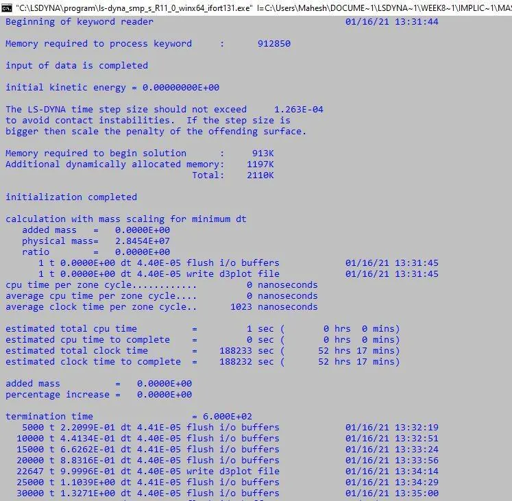

Trail 8 : for this trail dt2ms value is -5.0E-05

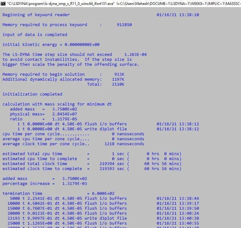
As we can see mass percentage starts to increase at 0.01% for this trail and the problem time is still huge.

Trail 9 : For this trail dt2ms value is -6.0E-05

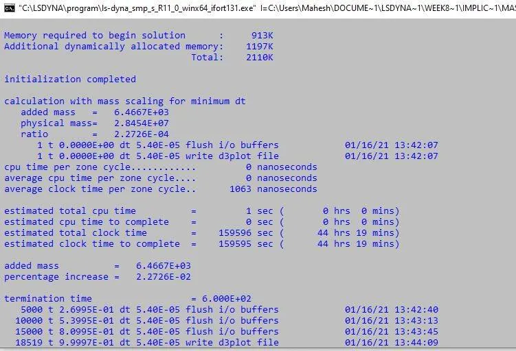
Trail 10 : For this trail dt2ms value is -7.0E-05.

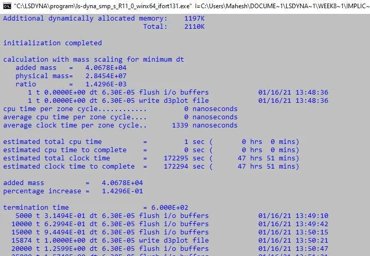
Trail 11 : For this trail dt2ms value is -9.0E-05.

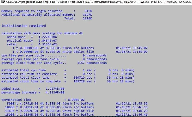
Here we can see that mass percentage(4.31%) is close to the 8% and problem time is reducing.

Trail 12 : For this trial dt2ms is -1.0E-04

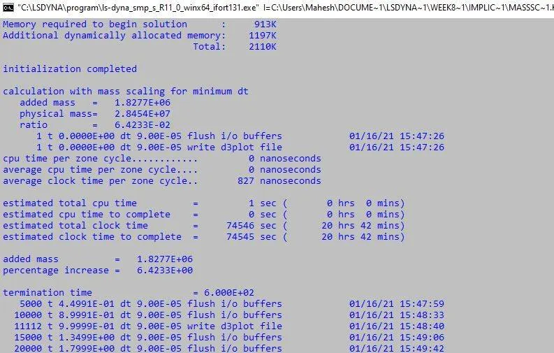
Here we can see that mass pecentage is very close to the 8% so we need to increase the dt2ms with samll values.

Trail 13 : For this trail dt2ms value is -1.5E-04

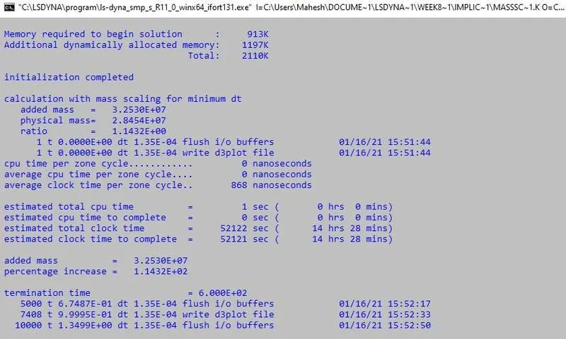
Here mass percentage is 100% which is more than we need and now we can consider that dt2ms value must be less -1.5E-04 and greater than -1.0E-04.

Trail 14 : For this trail dt2ms value is -1.03E-04

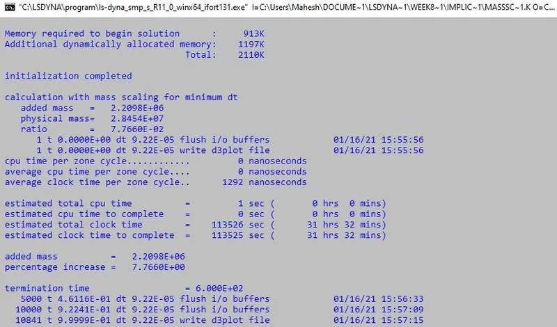
For this trail we can see that we almost to the 8% 0f mass so the dt2ms value must be lees than this.

Trail 15 : This is the final trail for the mass scaling dt2ms and tssfac values are -1.029E-04 and 0.9.

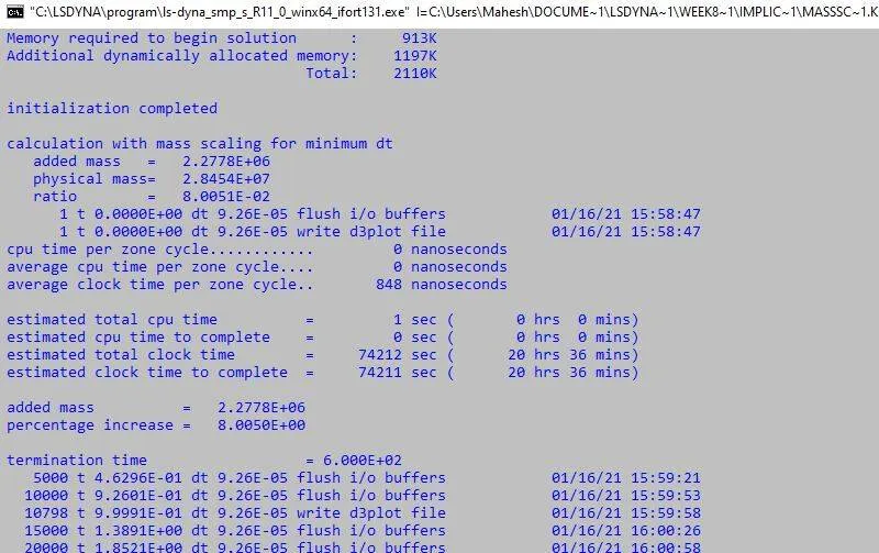
Finally for this dt2ms value we got the mass percentage as 8% and the problem time is reduce to 20 hrs.

Step 4 : Now we need to check for same dt2ms value but different tssfac values. dt2ms values are 0.8, 0.7, 0.6.

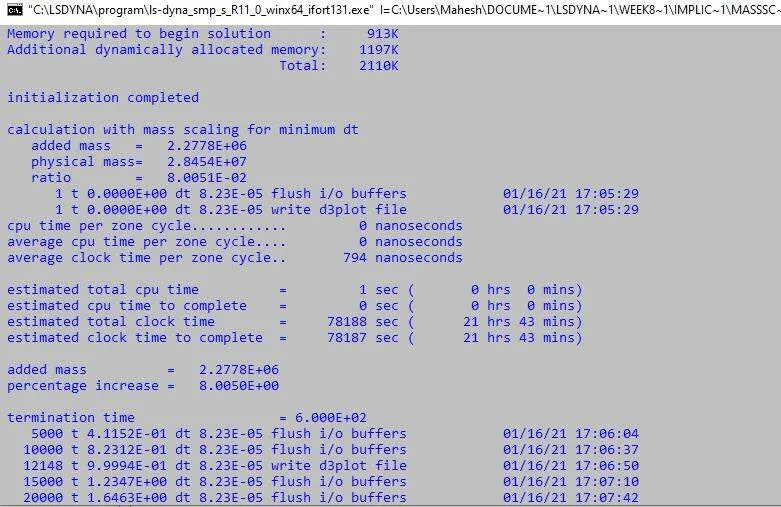
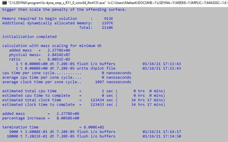
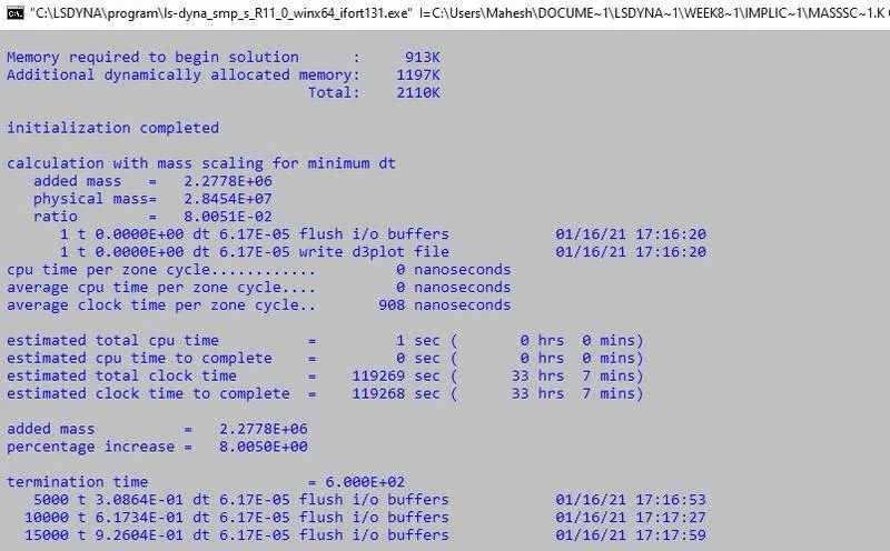
As we can see when the tssfac value is reduced then there is raise in the problem time.

Step 5 : Now we have to compare the explicit and implicit analysis, above all trails are done in the explicit analysis. To do in implicit analysis we need to add some keycards like implicit auto, implicit general, implicit solver and implicit solution.

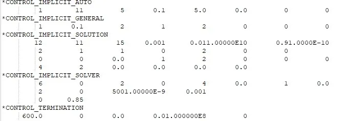
Now we have the implicit cards and run the file in the ls manager with two different dt2ms values -3.50E-05 which is default value and -1.0248E-05 which gives the mass percentage of 8%.

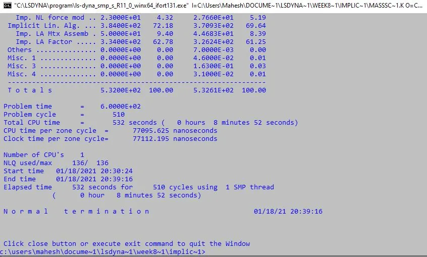
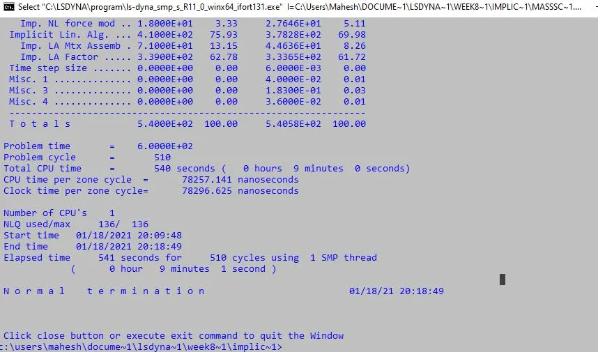
As we can see the both final problem time is reduced ccomparing to the explicit analysis.

Step 6 : Now we have to plot the histogram of dt2ms and runtime of trails using the Ms Excel softare.

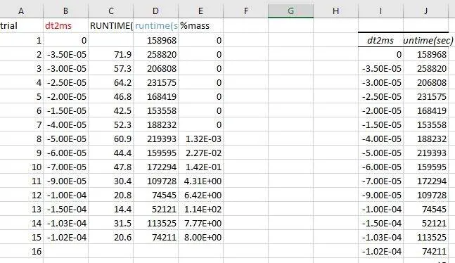
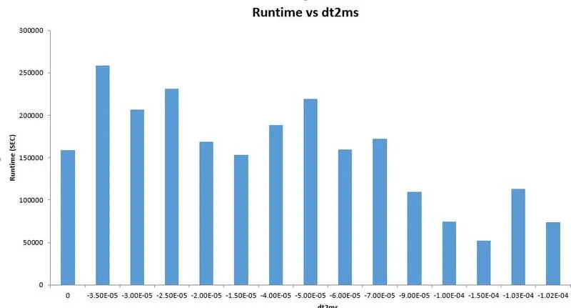
From the histigram we can see that dt2ms value is affecting the run time of the sover and highest run time is occured at the default value -3.5E-05 and least occured at the -1.5E-05.

Conclusion :

Thus we have find out the dt2ms or mass scaling value for 8% with the help of trail and error method and we have plotted the graph for dt2ms and Runtime.