Week 3 - Solving second order ODEs

1. Aim:

To write a program to solve the 2nd order ODE and animate the motion of simple pendulum.

2. Governing equations:

1. The governing equation used here is 2nd order ODE representing the motion of simple pendulum:
   • `(d^2theta)/(dt^2)+(b/m)*((d theta)/dt)+(g/l)*sintheta = 0`
     • where
       1. b = Damping co-efficient.
       2. m = Mass of the ball in kg.
       3. g = Acceleration due to gravity(9.81 m/sec^2)
       4. l = Length of the pendulum in meters.
       5. theta = Angle in radians.
2. Trignometric relations:
   • `sintheta = (opps ite)/(hypotun use)`
   • `cos theta = (adjesent)/(hypotun use)`

3. Objectivce of the project:

1. To execute the program to solve for 2nd order ODE.
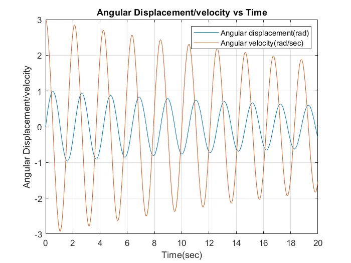
2. To plot the time versus angular displacement.
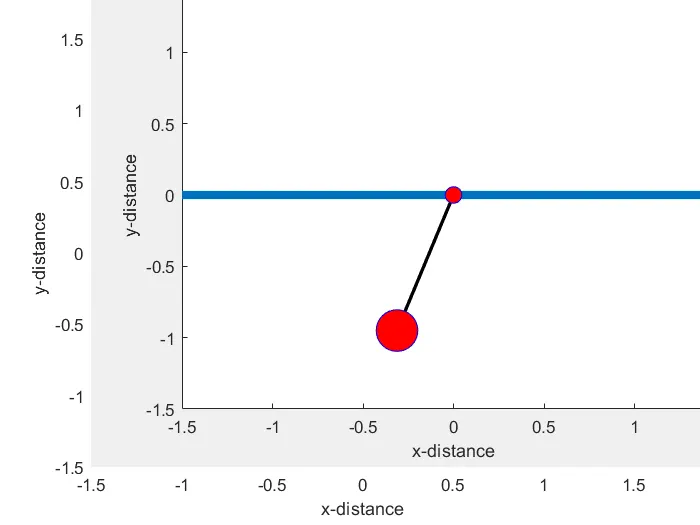
3. To animate the motion of simple pendulum for given initial conditions.

4. Body of the content:

1. The body of the program contains the
   1. Clearing command,
   2. Defined inputs,
   3. Defining the function,
   4. Solving for the given ODE by 'ode45' command,
   5. Plotting the Time versus Angular displacements and animating the motion of the simple pendulum.
2. Software used is MATLAB (Language - c/c++)

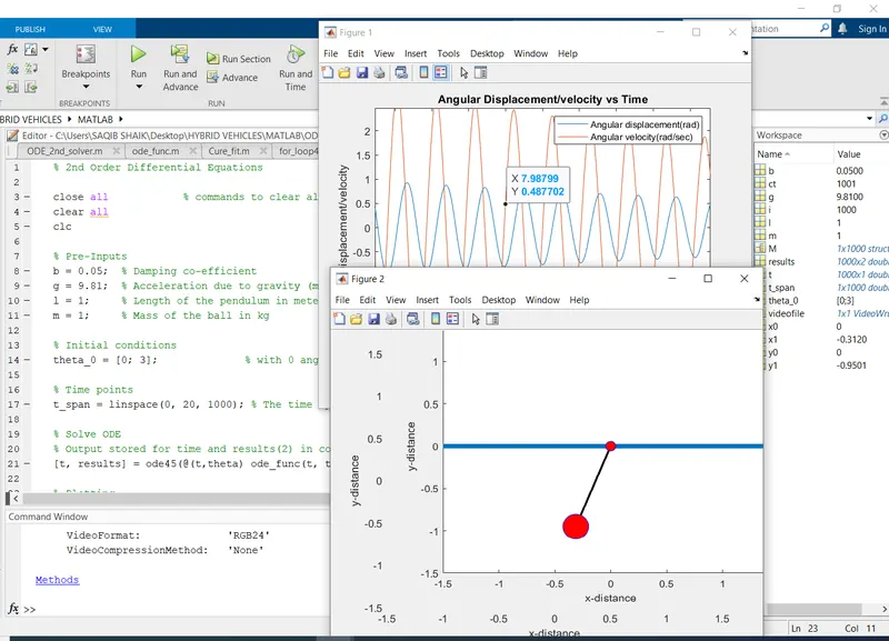
3. % 2nd Order Differential Equations
   
   close all            % commands to clear all the garbage values and close any program or figure
   clear all 
   clc
   
   % Pre-Inputs
   b = 0.05;  % Damping co-efficient
   g = 9.81;  % Acceleration due to gravity (m/s^2)
   l = 1;     % Length of the pendulum in meters
   m = 1;   % Mass of the ball in kg
   
   % Initial conditions
   theta_0 = [0; 3];              % with 0 angualar displacement (rad) and a angular velocity of 3 rad/sec
   
   % Time points
   t_span = linspace(0, 20, 1000); % The time span/limit is used in solving the ODE
   
   % Solve ODE
   % Output stored for time and results(2) in columns
   [t, results] = ode45(@(t,theta) ode_func(t, theta, b, g, l, m), t_span, theta_0);  % ODE command and predefined function is called.
   
   % Plotting
   figure(1)            % Time v/s angular displacements.
   plot(t,results(:,1))
   hold on
   plot(t,results(:,2))
   ylabel('Angular Displacement/velocity')
   xlabel('Time')
   legend('Angular displacement','Angular velocity')
   
   ct=1;                            % For updating the frames.
   figure(2)                        % Pendulum postion of every angle.
   for i = 1:length(results(:,1))   % Till the length of the angular displacement
       x0 = 0;                      % Defining the piviot point of the pendulum
       y0 = 0;
       x1 = l*sin(results(i,1));    % Calculating the position of the End of the pendulum 
       y1 = -l*cos(results(i,1));
       plot([-1.5 1.5], [0 0],'linewidth',10)      % Plotting the reference anchour of the piviot  
       hold on
       plot([x0 x1], [y0 y1],'linewidth',2,'color','k') % Plotting the pendulum
       plot(x1,y1,'o','Markersize',20, 'MarkerFaceColor','r','color','b')
       plot(x0,y0,'o','Markersize',7, 'MarkerFaceColor','r','color','r')
       axis([-1.5 1.5 -1.5 1.5])                        % Pre defining the axis dimensions
       pause(0.001)                                     % Pausing the figure
       xlabel('x-distance')
       ylabel('y-distance')
       
       M(ct)=getframe(gcf)                              % Storing the frames in the M using the getframe command gcf- get current command
       hold off
       ct=ct+1;                                         % Updating the count value every time loop completes
   end
   movie(M)                                             % Creating the movie ussing frames array M
   videofile = VideoWriter('Simple_pendulum.avi')       % Creating the videofile for writing the frames into it.
   open(videofile)                                      % Opening the videofile.
   writeVideo(videofile, M)                             % Writing to the video.
   close(videofile)                                     % Closing the videofile.
   

4. The previous stored values are cleared using the commands.
5. The predefined data is given as input.
6. Intial conditions are defined angular displacement as zero and angular velocity as 3 rad/sec.
7. The command ode45 is used to solve the 2nd order ODE along with the predefined function.
8. The output is with respect to time for two results i.e angular displacement and angular velocity.
9. The trignometric equations are used to solve the position of the pendulum and is plotted.
10. Every frame of this plot is saved in array called 'M'.
11. The ball and the piviot are done using 'Marker' command with different sizes and color.
12. The variation of the angular velocity and angular displacement is plotted against the time for 20 sec.
13. The 'movie' command is used for the array'M' to make a video.
14. The videofile id is assigned to the video and name as 'Simple_pendulum', using the VideoWriter command to open as write.
15. Open command is used to open the videofile.
16. The 'writeVideo' command is used to write the frames into it.
17. Then by using the close command the videofile is closed.

18.  % Function to solve ODE
     
     function [dtheta_dt] = ode_func(t, theta, b, g, l, m) % Defining the function and the inputs
     
     theta1 = theta(1)
     theta2 = theta(2)
     dtheta1_dt = theta2;                                % Assigning the values of theta.
     dtheta2_dt = -(b/m)*theta2 - (g/l)*sin(theta1);     % Equation to solve the ODE.
     dtheta_dt = [dtheta1_dt; dtheta2_dt];               % Storing the two outputs.
     end
    

19. The above code represents the program to solve the ODE used in the ode45 command.
20. First the theta values are assigned so to convert the second order differential equation into first order differential equation.
21. Then by using the equation and the predefined input and time span array the converted ODE is solved.

5. Results:

1. After the execution of the program we have a graph and a animated video.
   • 
2. The graph shows the variation of the angular displacement with respect to time.
   • 
3. This animation shows the motion of simple pendulum obtained by solving 2nd order differential equation:
   • 

6. Conclusions:

1. The program is successfully executed to solve the 2nd order differential equation.
2. The variation of the angular displacement and angular velocity are studied by using the graph angular displacement/velocity versus the time.
3. The animation shows the motion of the simple pendulum using the 2nd order differential equatiion.
4. The pendulum doesnt come to rest in 20 sec.

7. References:

1. Michael C. Agarana, Esther T. Akinlabi,
   Analytical modelling of driven pendulum with small angular displacement using Undetermined Coefficients Method,
   Procedia Manufacturing,
   Volume 35,
   2019,
   Pages 689-697,
   ISSN 2351-9789,
   https://doi.org/10.1016/j.promfg.2019.06.010
   (https://www.sciencedirect.com/science/article/pii/S2351978919307358)
2. Jin Wang, Qilong Xue, Lixin Li, Baolin Liu, Leilei Huang, Yang Chen,
   Dynamic analysis of simple pendulum model under variable damping,
   Alexandria Engineering Journal,
   Volume 61, Issue 12,
   2022,
   Pages 10563-10575,
   ISSN 1110-0168,
   https://doi.org/10.1016/j.aej.2022.03.064
   (https://www.sciencedirect.com/science/article/pii/S1110016822002393)