Week 9 - Parametric study on Gate valve.

Aim: To perform the simulation on the gate value for different levels of the opening using the parametric study.

Objective:

1. Importing and cleaning the geometry.
2. Setting the opening of the gate valve and extracting the fluid volume.
3. Meshing the geometry.
4. Running the mesh independency test.
5. Running the simulation.
6. After a single run of simulation switching to the parametric study with different percentages of opening.
7. Analyzing the results and concluding the inferences obtained.

Theory:

1. Flow co-efficeint(Cv):
   • It is the relative measure of efficiency which describes how efficiently the fluid flows across the valve.
   • It gives the relation between the pressure drop and the corresponding flow rate.
   • It can be given as:
     • `Cv = Q*sqrt((SG)/(dP)`
     • were `dP` = Pressure drop across the inlet and the outlet (measured in psi).
     • SG = Specific gravity.
     • Q is the mass flow rate (Gallons per minute).
   • It may also be said as the amount of fluid (water) flowing across in gallon per minute (US) at 60 F when the pressure difference is 1 psi across the valve opening.
2. Flow factor(Kv):
   • It defines the amount of the fluid flow in `m^3/h` when the valve is fully opened and the pressure difference is `1 (kgf)/(cm^2)`.
   • It can be given as:
     • `Kv = Q*sqrt((SG)/(dP))`
     • were Q is the mass flow rate in `m^3/h`
     • SG is the specific gravity of the fluid. (For water - 1)
     • dP is the pressure difference across the valve in bars.
   • The flow factor can also be calculated as:
     • Kv = 0.865*Cv.
3. Substituting all the values obtained after the simulation in the above equation will give us the values of flow factor and flow co-efficient.

Content of the body:

1. Open the Ansys Fluent and Spaceclaim for the geometry preparation.
2. Import the geometry using the file open option or just drag and drop:
   • 
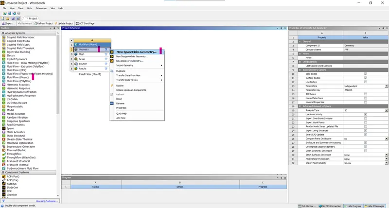
   • Importing the geometry.
   • 
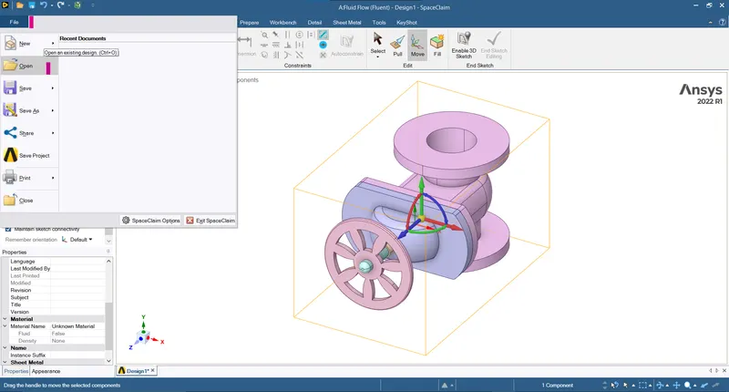
3. After checking for any errors.
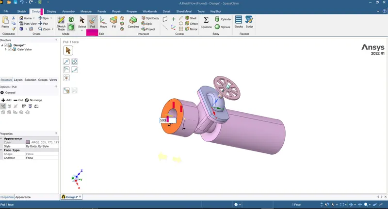
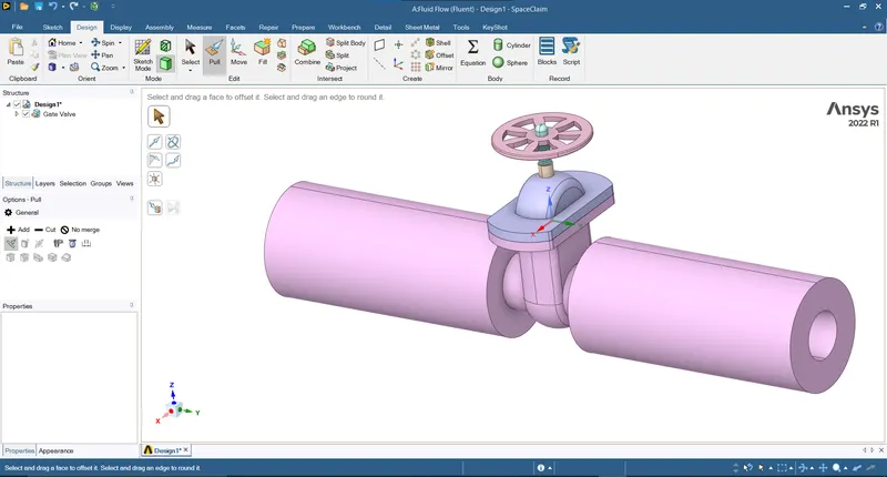
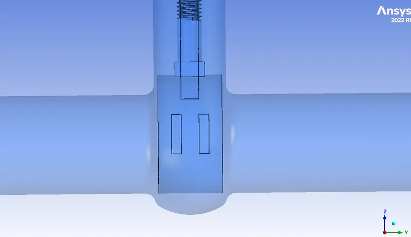
4. As the outlet and the inlet are short we are going to elongate them using the pull tool (Design > Pull > select the face > Extend):
   1. 
   2. After the elongation.
   3. 
5. Displacing/moving the value accordingly (Design > Move > select the valve body > give the displacement > ok):
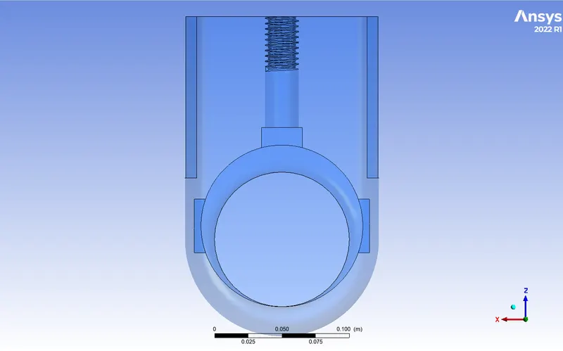
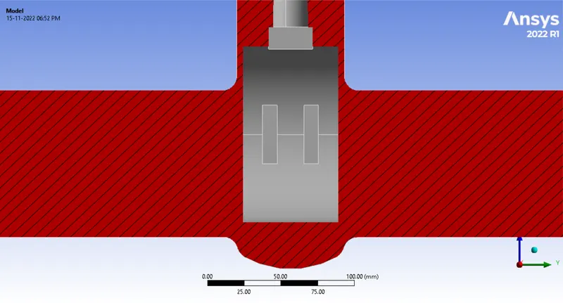
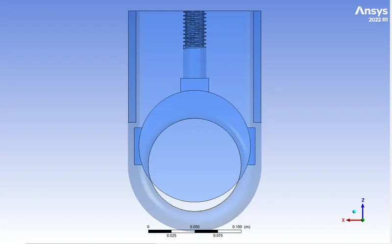
   1. As we can see the diameter of the tube is 10mm.
   2. 
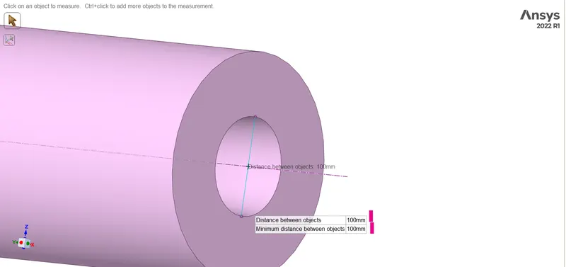
   3. At zero percentage of opening:
   4. 
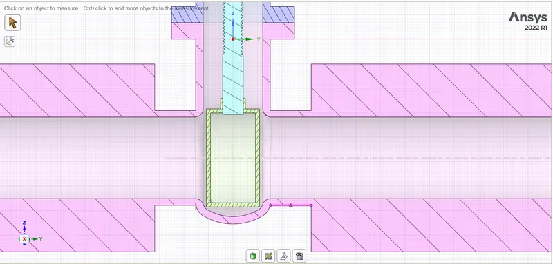
   5. Now increasing the opening distance to 10 mm (Design > Move > select the component > Move to distance > Ok):
   6. 
   7. 
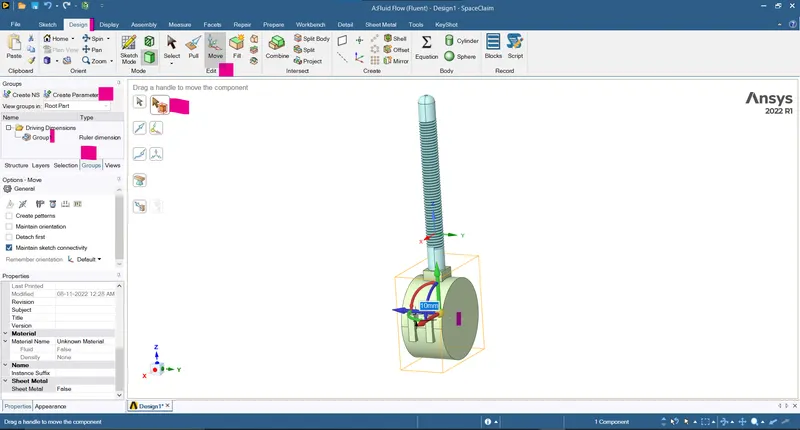
   8. After moving for 10mm or 10%:
   9. 
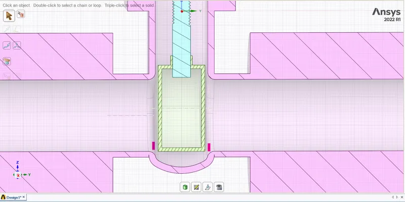
   10. Here we also created the parameter with the driving dimension for components named under Group1 (here gate) through which the opening can be altered without any much difficulty (Groups > Create parameters > give the dimension).
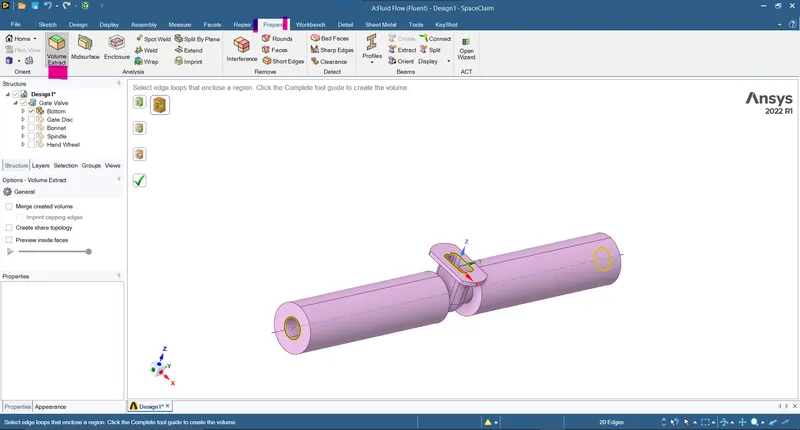
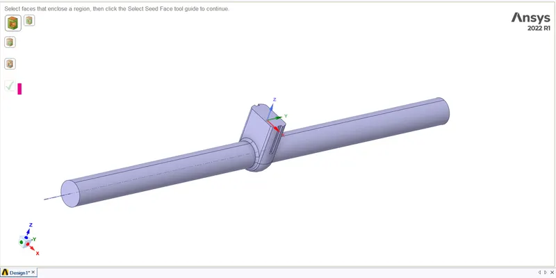
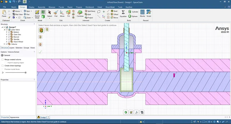
6. Extracting the fluid volume (Prepare > volume extract > select the edges > Ok):
   1. Selecting the edges:
   2. 
   3. After:
   4. 
   5. 
   6. Now supress the component for physics which are not needed in the flow analysis (Right click > suppress for physics):
   7. 
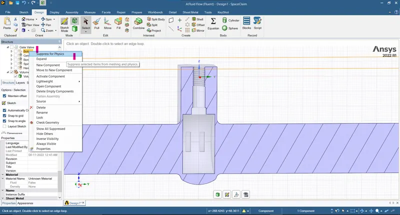
   8. Now whenever the displacement of the gate is changed we need to update the fluid volume as it changess as per the displacement of the gate (Right click on the volume > Update volume body by context):
   9. 
   10. 
   11. 
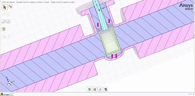
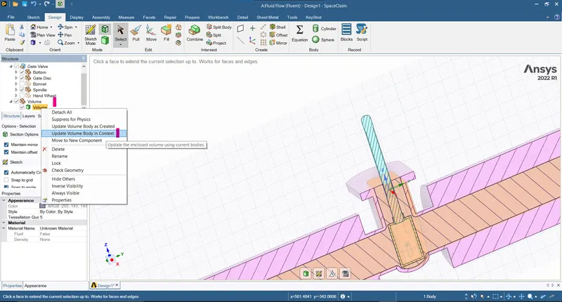
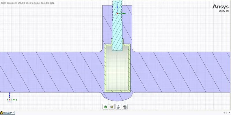
7. Meshing:
   1. Open the meshing:
   2. 
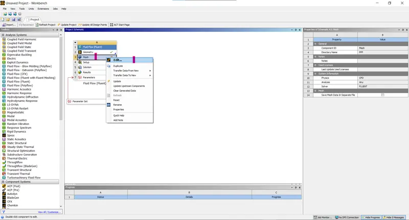
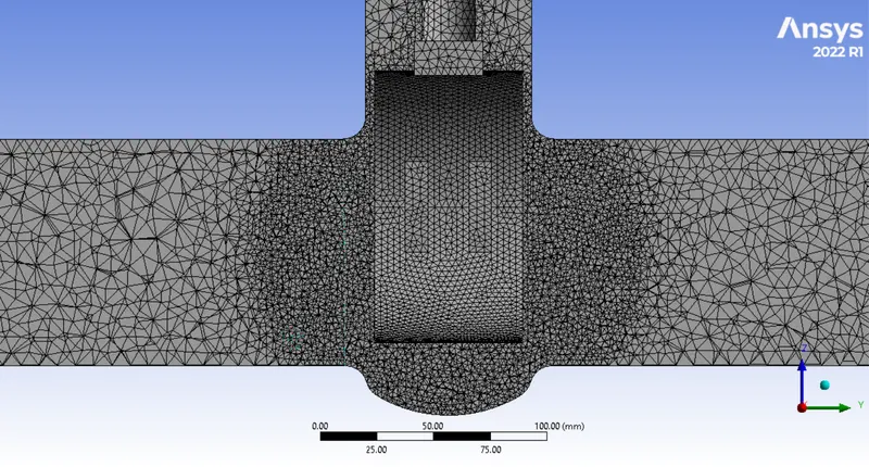
   3. Generate the mesh (Mesh > Right click > Generate mesh):
   4. 
   5. 
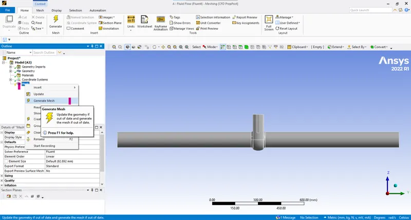
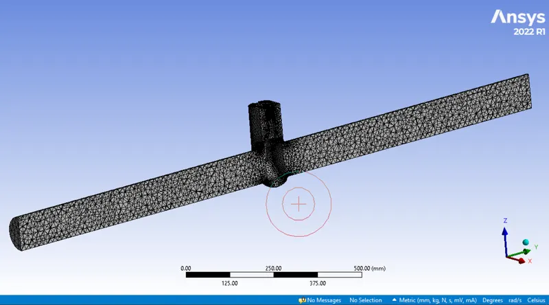
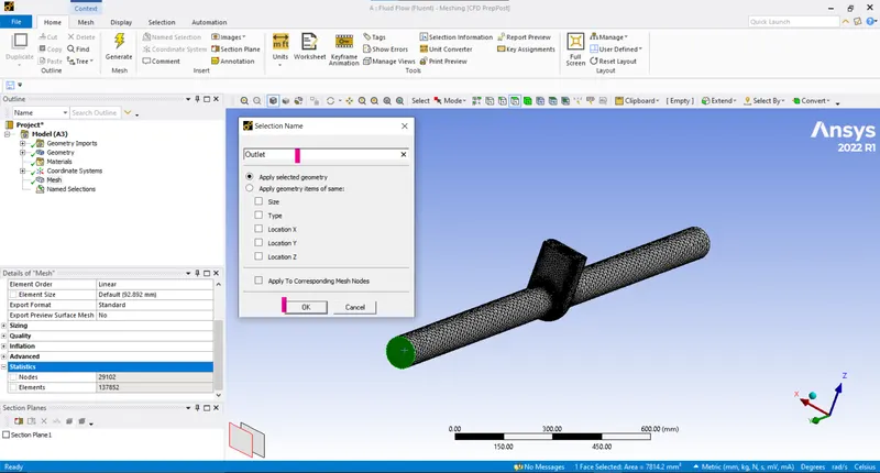
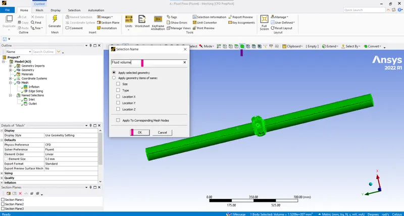
   6. Now naming the faces (Select the face > Create the named selection > Ok):
   7. 
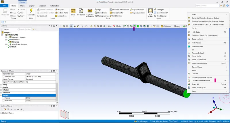
   8. Inlet:
   9. 
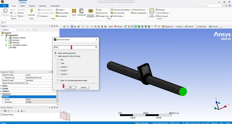
   10. Outlet:
   11. 
   12. Fluid volume:
   13. 
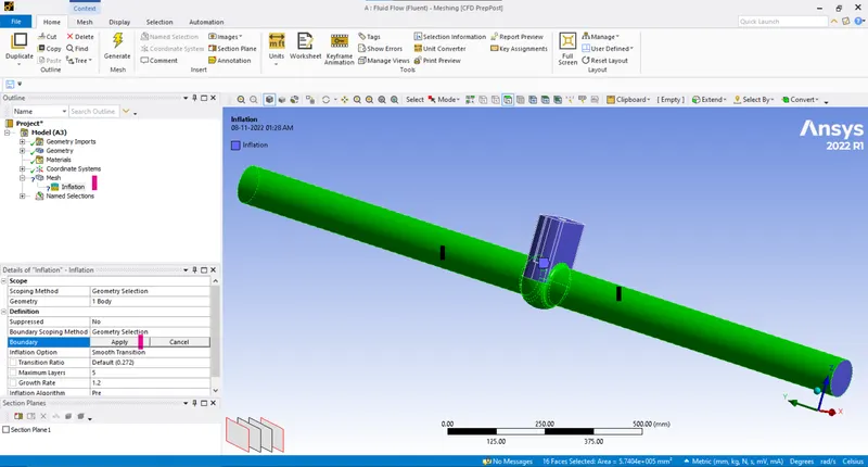
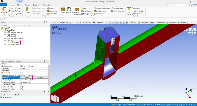
   14. Creating the inflation layers (Insert > Inflation > Select the geometry > Select the boundary > Ok):
   15. Selecting the body and the faces:
   16. 
   17. 
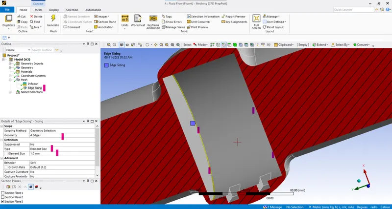
   18. Performing the edge sizing (Insert > Sizing > select the edges > Type > Element size > Give the size > 1mm > Ok):
   19. 
   20. 
   21. 
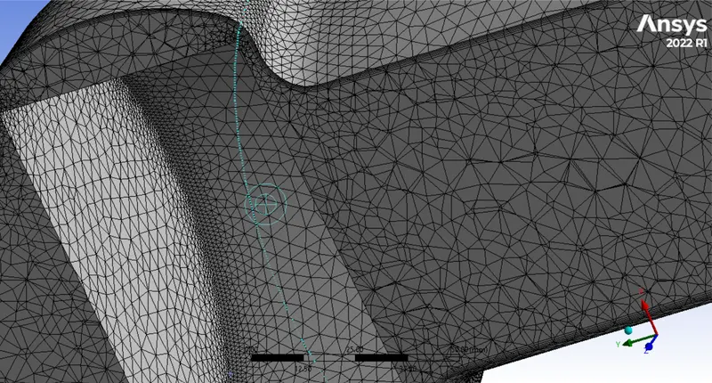
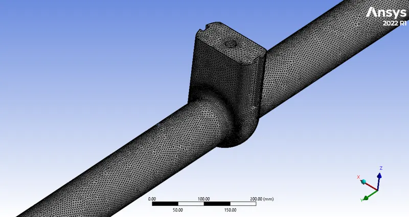
   22. Update the mesh (Mesh > update):
   23. 
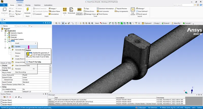
   24. Now as the meshing is complete we can move to the setting up the physics and boundary conditions.
8. Setup:
   1. 
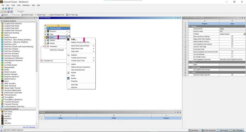
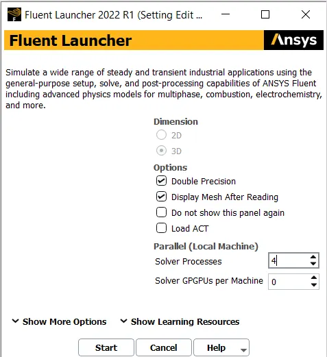
   2. Double precision is enabled.
   3. 
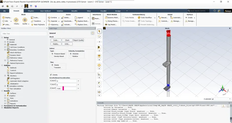
   4. Here the gravity is enabled as here the influence of gravity is taken into consideration (ngative z direction):
   5. 
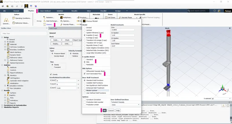
   6. Viscous model - k-epsilon RNG model with swirl dominated flow is selected as this model is suitable for the flow in tubes and were the swirls are formed (Physics > viscous > model select the model > Ok):
   7. 
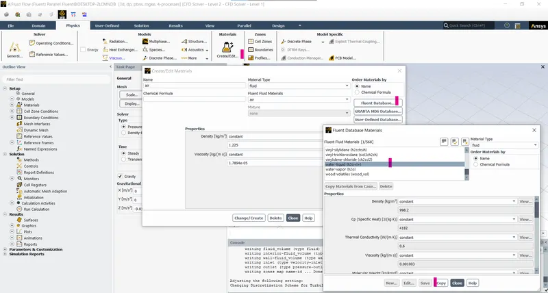
   8. Now add the materials remove the default material air and add water (Materials > Fluent database > Fluid > Select the fluid material > Copy):
   9. 
   10. Assigning the materials to te cell zones (cell zone > select the zone > Type > Edit > assign the fluid > Apply):
   11. 
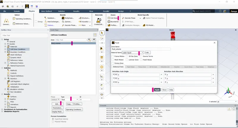
   12. Here the fluid used is water.
   13. Define the boundary conditions (Boundary conditions > Select the zone > Give the magnitude and direction > Ok):
   14. 
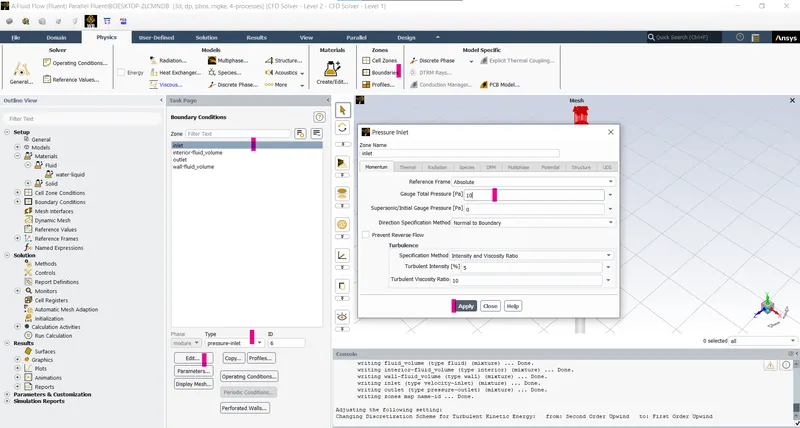
   15. Here the inlet is pressure based inlet with pressure of 20 pascals at the inlet:
   16. 
   17. The pressure here is 20 Pascals at the inlet.
   18. Outlet is the pressure outlet at gusage pressure equal to zero.
   19. 
   20. Defining the reports (Solution > Definition > New > Surface reports > Mass flow rate > At outlet > Create output parameter > Ok):
   21. 
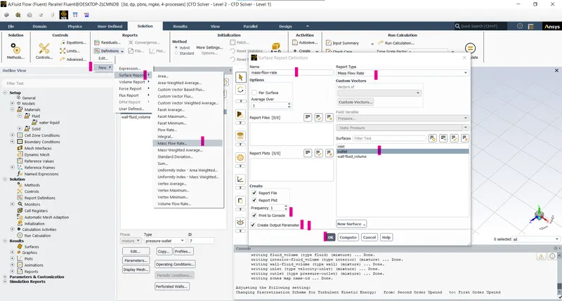
   22. Here the create the output parameter is created as we are running the parameteric study simulation in this prospect the parameter will be update at the parametric set.
   23. Initializing the setup using the hybrid initialization as it is a steady state problem:
   24. 
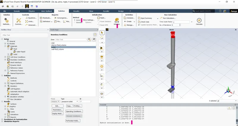
   25. Now adding the contours for the visualization of the velocity accross the midplane (Results > Contours > Velocity contour > Select the plane > save/display):
   26. Create the plane in zy direction (Results > Create > plane > zy > Ok):
   27. 
   28. 
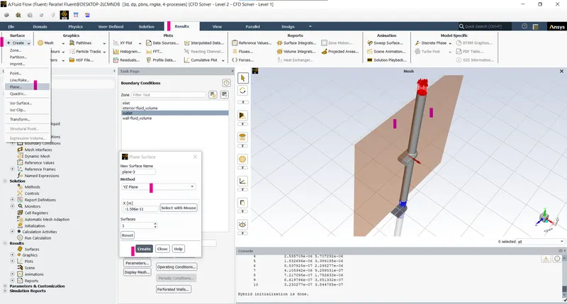
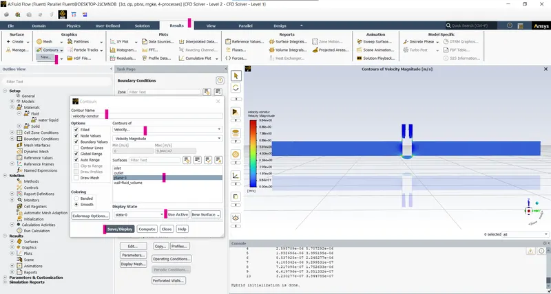
   29. The active view is used.
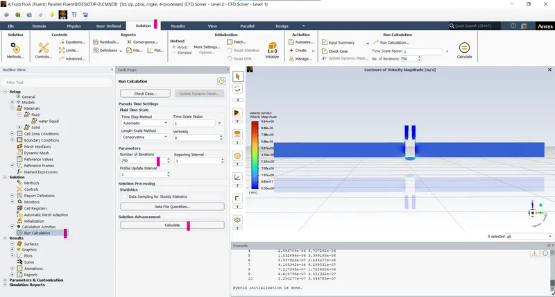
   30. Now run the simulation for 750 iterations (Run calculation > set the number of iterations > Calculate):
   31. 
   32. Using the parametric set:
   33. 
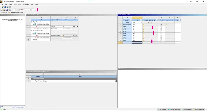
   34. Here add the parameters for the defined group (From 10mm to 80mm):
   35. 
   36. Add the parameter for the group by entering the variable for each state by defining the value in the below section of the predefined set.
   37. As the simulation is complete we can proceed to the post-processing.
   38. The parameter set option is used when all the major physical and boundary conditions remain the same and only certain parameters, physical or boundary conditions are altered for a new study to be performed at this point the parametric study is done to run the study for different cases using the almost same setup conditions and study the effect of the parameter varied.
   39. The duplicate of the case also can be done to run the study but in the parametric study the solution can be arranged or setup in order to execute one after another without every time running the setup as in the case of duplicate.
9. Post-processing:
   1. Open results in the Fluent.
   2. 
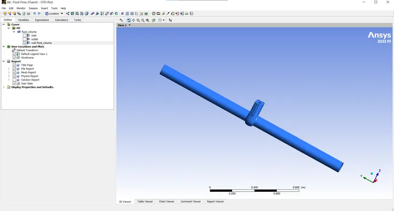
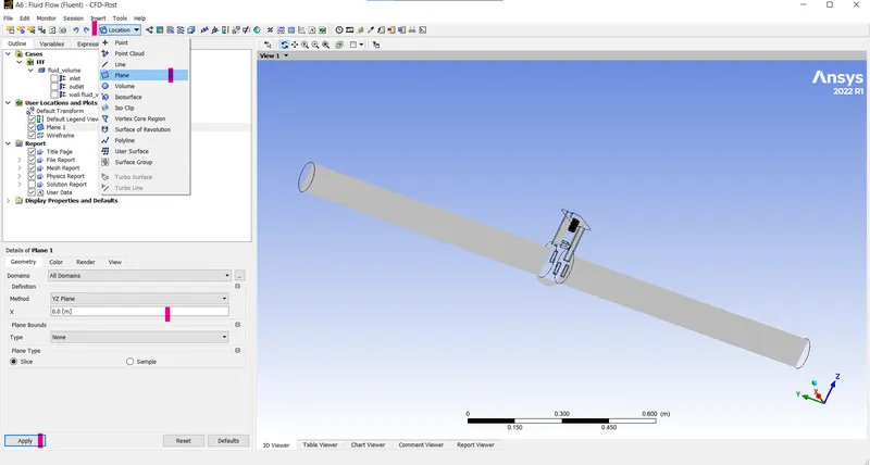
   3. To visualize the variable parameters like pressure, velocity etc. we must include a plane in yz direction so to study the behaviour of the fluid (Location > Plane > select the axis for plane > Apply):
   4. 
   5. Now for the pressure distribution change the variable to pressure (Plane > color > Variable > pressure > Apply):
   6. 
   7. 
   8. 
   9. 
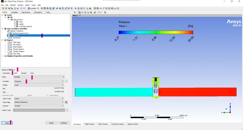
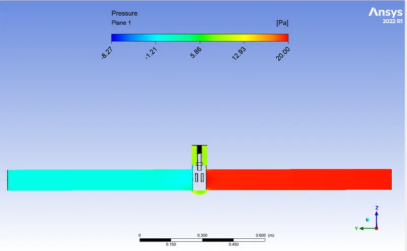
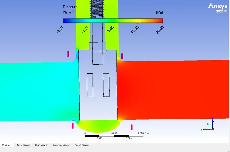
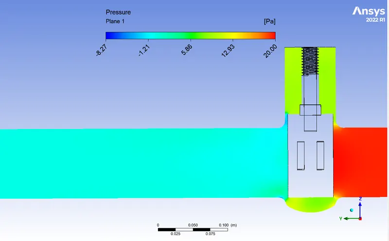
   10. As the valve is only 10% open it creates a more closed condition for the valve which means it restricts the flow creating the high-pressure region to the side of the inlet and comparatively less pressure towards the outlet side.
   11. It may be put in as the valve is closed it obstructs the flow creating the high-pressure regions before the valve and as the fluid passes the valve it undergoes minor throttling effect as it increases the velocity and decreases the pressure.
   12. For the velocity distribution the valve tube change the variable to velocity (Plane > color > Variable > Pressure > Apply):
   13. \
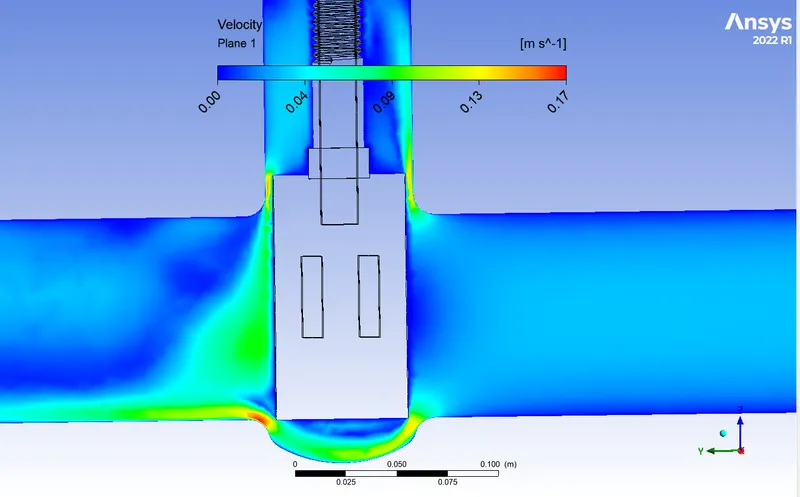   14. It can be seen that the fluid behind the valve is at high pressure and low velocity and the valve creates a throttling effect that pushes the fluid to the other side increasing the velocity and decreasing the pressure.
   15. The no-slip condition can be seen at the walls and the surfaces of the valve whose velocity is near to zero.
   16. As there is a very narrow gap for the fluid to escape at the valve gains velocity with the compromise on pressure creating the high-velocity regions at the narrow regions.
   17. We can observe the bulge at the bottom of the value which acts to suddenly increase the volume and decrease the pressure thus resulting in the high-velocity region and as the valve is verticle the pressure at the narrow opening acts as to push the fluid in radial directions so the fluid takes the pattern of the bulging volume during the low opening percentages.
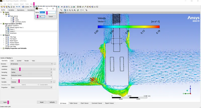
   18. For the visualization of velocity vectors of the fluid particle we need to add the vector plots (Add > Vector plot > Variable velocity > Ok):
   19. 
   20. 
   21. 
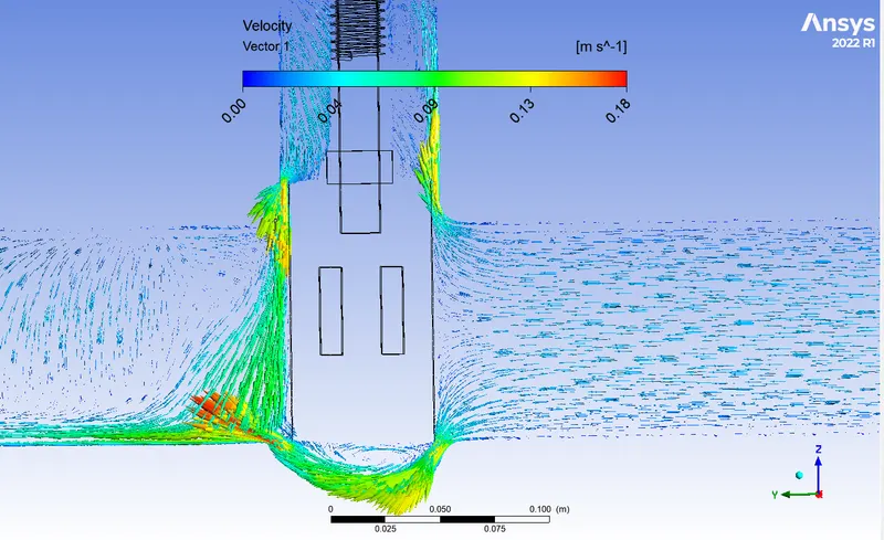
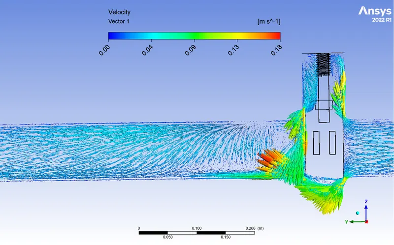
   22. The vector plot of the fluid particles depicts the velocity vectors of the fluid particle at various locations of the plane.
   23. It can be seen that the velocity is in the direction of the flow behind the valve and diverges at the valve location with an increase in the velocity at the sudden volume enlargements after the valve opening regions.
   24. After the fluid leaves the valve it has velocity in other directions which leads to the formation of the swirls in the many opening percentages and in some cases as above it causes the impingement on the pipe walls creating the area of high pressure and areas prone to corrosions.
10. To find the pressure at the inlet and outlet and mass flow rate we need to view surface reports (Solution > reports > Surface reports > Area weighted average > Select the variable > Compute):
    1. For the pressure at the inlet and outlet:
    2. 
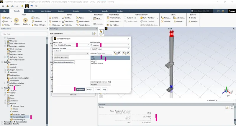
    3. For calculating the mass flow rate at the openings (Report > Fluxes > mass flow rate > select the openings > Compute):
    4. 
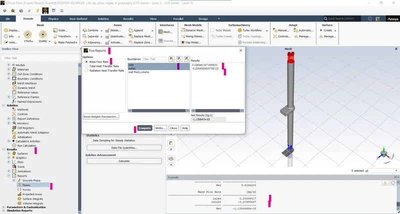
11. Now as we have the desired data we can calculate the flow co-efficient and flow factor by using the formula as explained above.

Results:

1. Note:
   1. Temperature contours - This represents the variation of temperature across the defined selection.
   2. Velocity contours - This represents the variation of velocity across the defined selection.
   3. Pressure contours - This represents the variation of pressure across the defined selection.
   4. Velocity vectors - This represents the magnitude and direction of the particle's velocity.
   5. Streamline - This represents the path followed by the particles and the color represents any selected property variation such as temperature, velocity etc.
   6. The percentage of opening represents the valve opened percentage.
2. Case-1 (10%):
   1. Openings:
      • 
      • 
   2. Residuals:
      
      • 
      • 
   3. Pressure contours:
      • 
      • 
      • The pressure contours represents the pressure variation in the geometry.
      • Since the valve is 90% closed which creates the high pressure region before the valve.
      • The pressure generated at the inlet is 19.6 pascals.
   4. Velocity contours and velocity vectors:
      • 
      • 
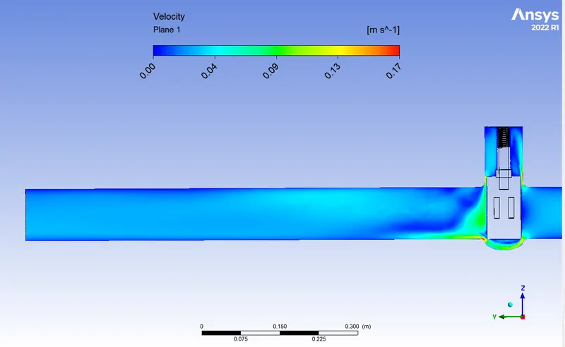
      • Velocity contours represent the variation of velocity.
      • As there is a small opening in the first case the pressure generated is more at the inlet the fluid escapes the valve at high velocity compared to the inlet.
      • It can be seen from the contours that the fluid has the highest velocity at the sudden constriction at the valve openings shown in red color.
      • 
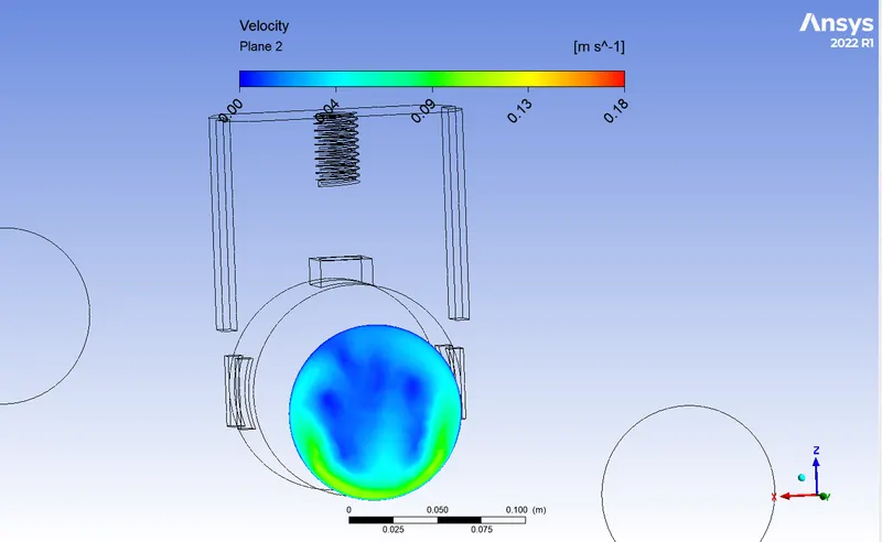
      • This velocity contours represents the variation of velocity across the crossection of the fluid flow.
      • We can observe that the velocity is more at the opening area of the valve as the pressure behind the valve pushes the fluid with higher velocity.
      • 
      • 
      • The above vector represents the velocity vector of the flow particles.
      • We can observe the flow diverges as near the valve at the inlet side and plunges in the openings areas with higher velocities.
      • The flow co-efficient is 61.2 and the flow factor is 52.9.
3. Case-2 (20%):
   1. Openings:
      • 
      • 
      • 
   2. Residuals:
      • 
      • 
      • 
   3. Pressure contours:
      • 
      • 
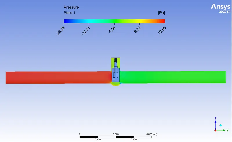
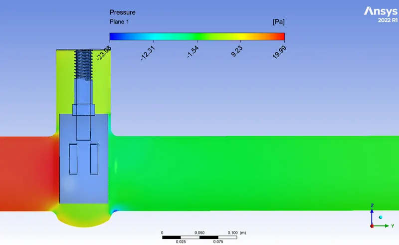
      • The pressure difference between the inlet and the outlet is reduced as compared to the 10% opening.
   4. Velocity contours and velocity vectors:
      • 
      • 
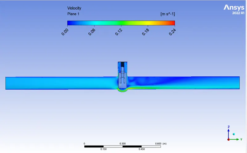
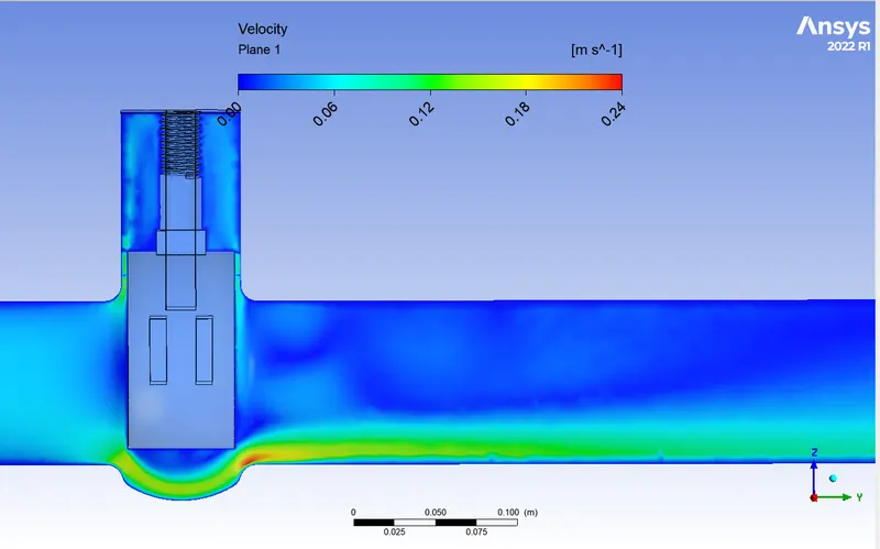
      • We can observe that there is more velocity for the fluid particles as they flow past the valve.
      • This forms large high velocity region in the lower region of the flow.
      • 
      • 
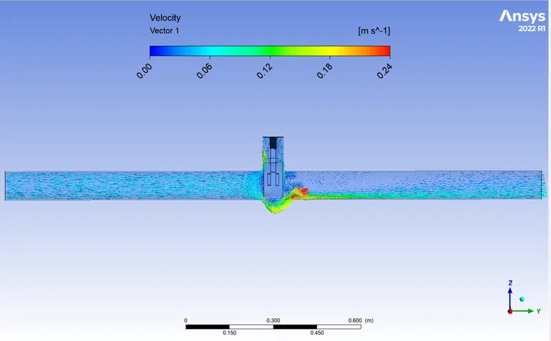
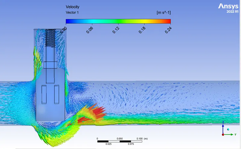
      • Due to the higher opening the velocity of the particles is more as the pressuredifference is less compared to the previous case.
      • We can clearly see the vortices forming after the valve opening.
      • 
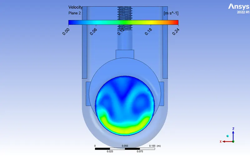
      • Here it ca be seen that due to more opening of the valve the high velocity region is more as compared to the 10% opening and the vortises are formed at the edges creating the swirling action.
4. Case-3 (30%):
   1. Openings:
      • 
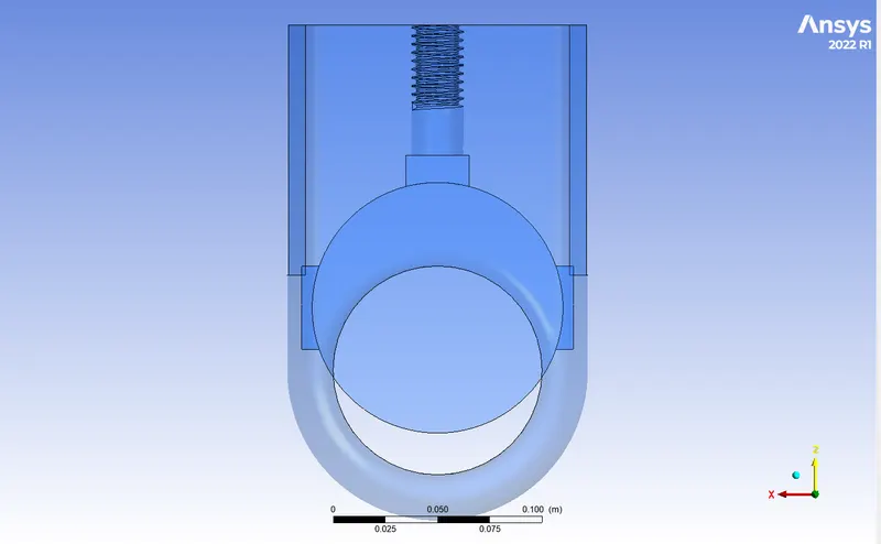
      • Her valve is opened to 30%.
      • The flow co-efficient is 102.0 and the flow factor is 88.22.
   2. Residuals:
      • 
      • 
      • 
   3. Pressure contours:
      • 
      • 
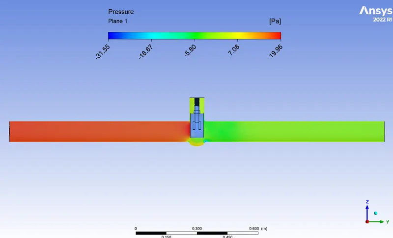
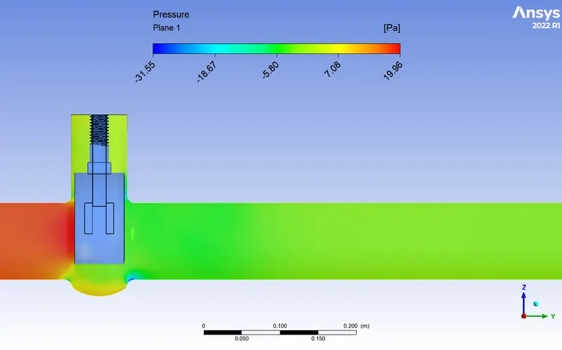
      • Since the obstruction is less compared to the last case the pressure difference is less between the inlet and the outlet.
   4. Velocity contours and velocity vectors:
      • 
      • 
      • 
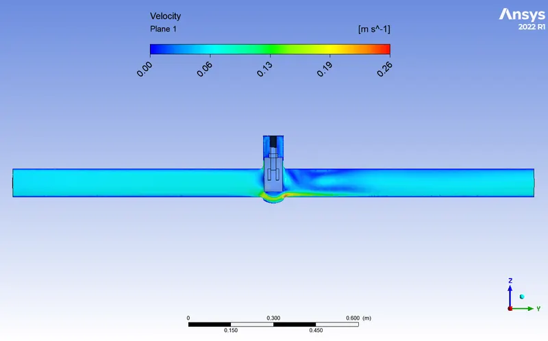
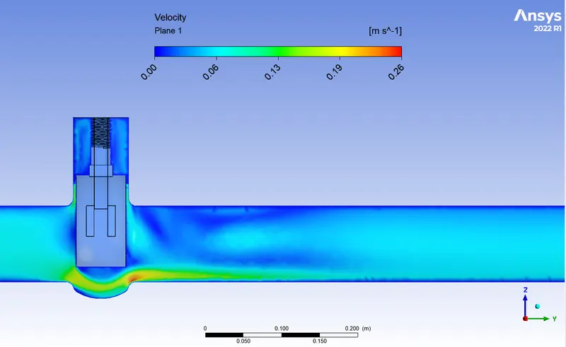
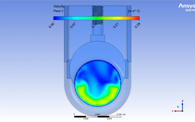
      • The high velocityregion region increases as the opening is increased.
      • The velocity at the outlet is more compared to the precious cases as the opening percentage is more resulting in the comparatively less pressure difference.
      • 
      • 
      • 
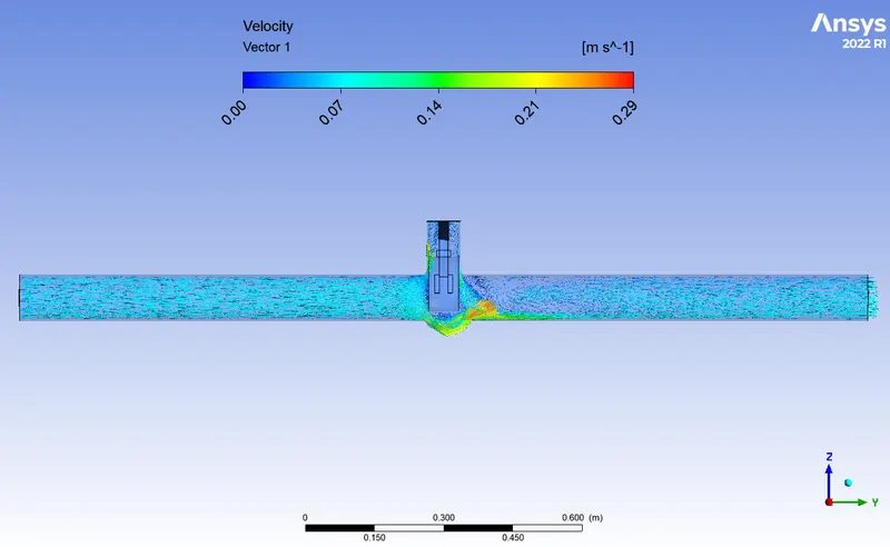
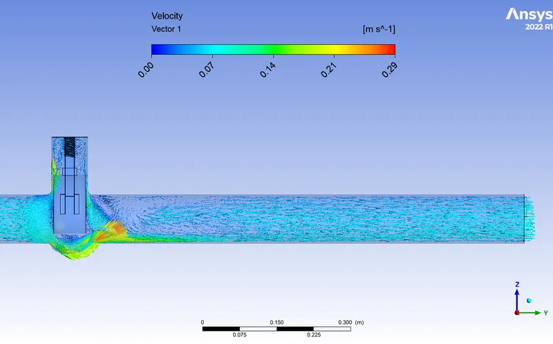
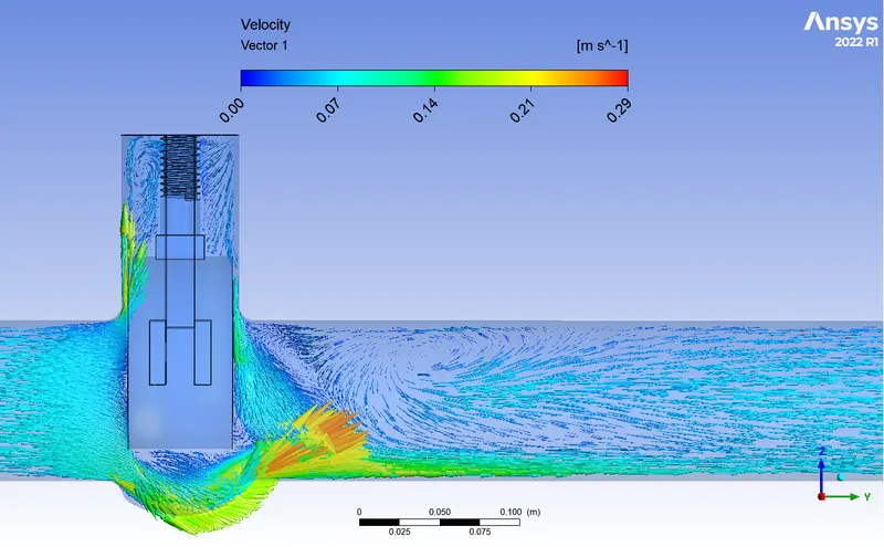
      • The velocity at the outlet is more as shown by the velocity vectors and the swirls are formed depicted by the vectors.
      • Here the flow co-efficient is 158.7 and the flow factor is 137.2.
5. Case-(40%):
   1. Openings:
      • 
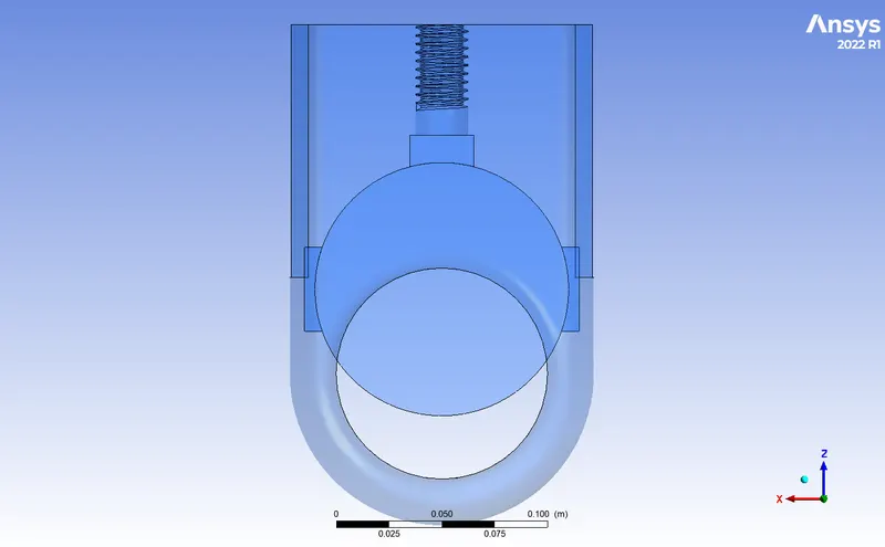
      • Here the valve is opened to 40%.
   2. Residuals:
      • 
      • 
   3. Pressure contours:
      • 
      • 
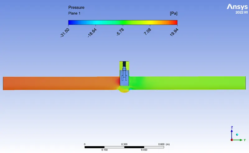
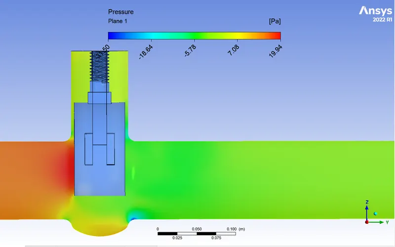
      • The pressure difference between he inlet and te outlet is 16.54 pascal which is less as compared to the previous cases.
   4. Velocity contours and velocity vectors:
      • 
      • 
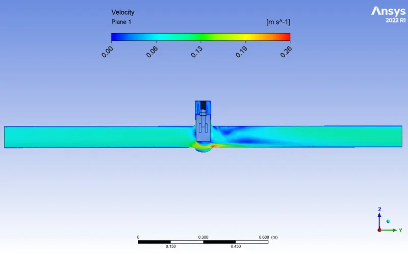
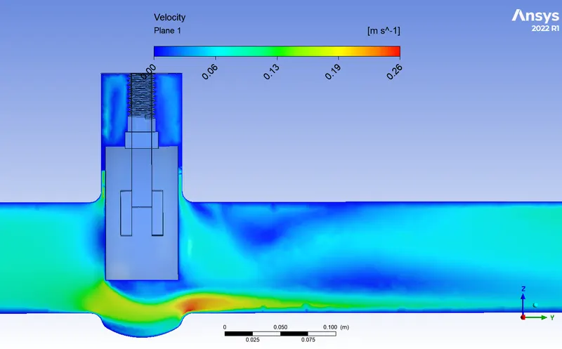
      • We can see that the high velocity region dessipates as it flow no like the previous case were the high velocity region was prominent.
      • The velocity is higher at the outlet as compared to the previous cases.
      • 
      • 
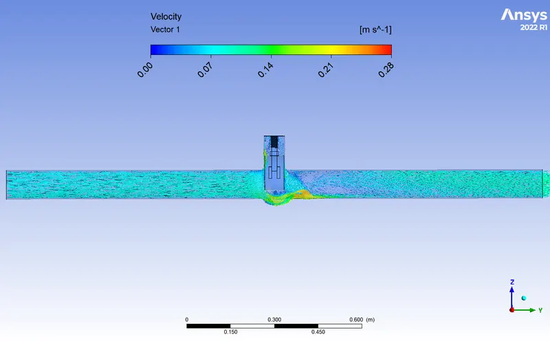
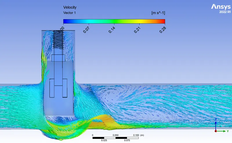
      • Here the velocity magnitude and the direction can be seen and the vortices formed can also be visualized.
      • 
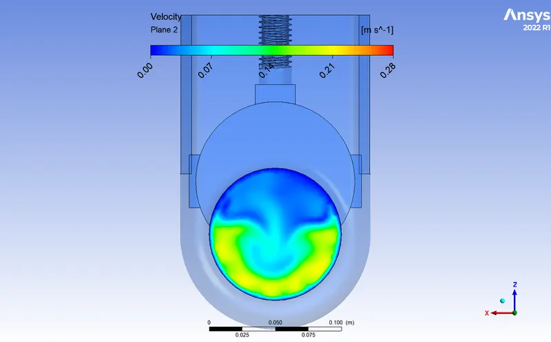
      • Here in the cross-sectional view of the velocity profile it can be seen that how the flow behave as it exits the valve area creating the swirls.
      • The flow co-efficient is 210.1 and the flow factor is 181.7.
6. Case-5 (50%):
   1. Openings:
      • 
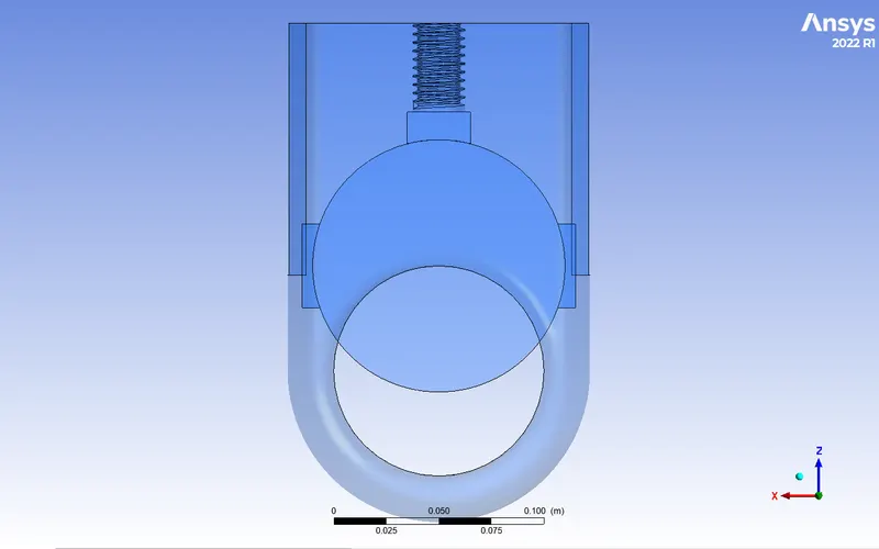
      • Here the opening is 50%.
   2. Residuals:
      • 
      • 
      • 
   3. Pressure contours:
      • 
      • 
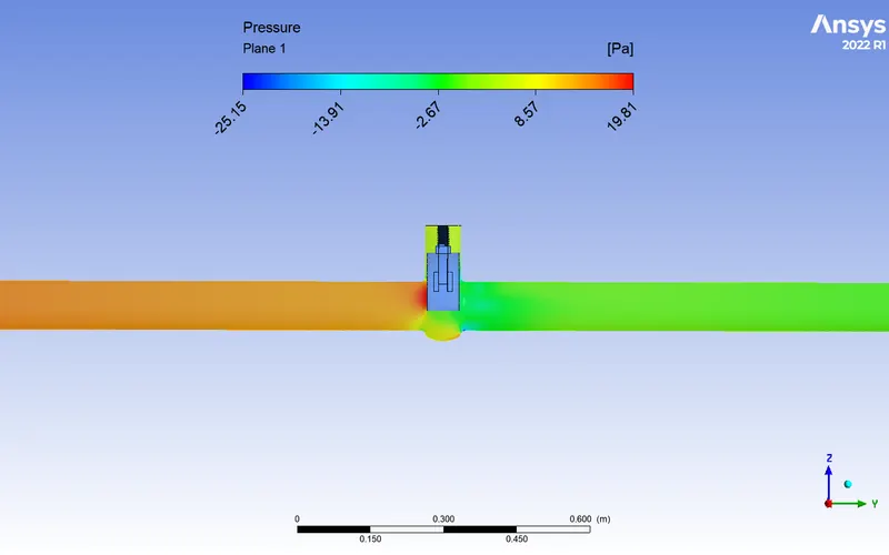
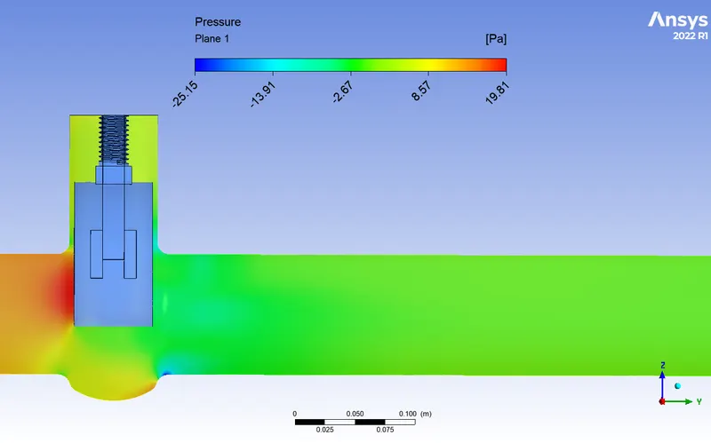
      • Here as usual there is high pressure at the inlet side than outlet but the pressure difference is less compared to the other cases.
   4. Velocity contours and velocity vectors:
      • 
      • 
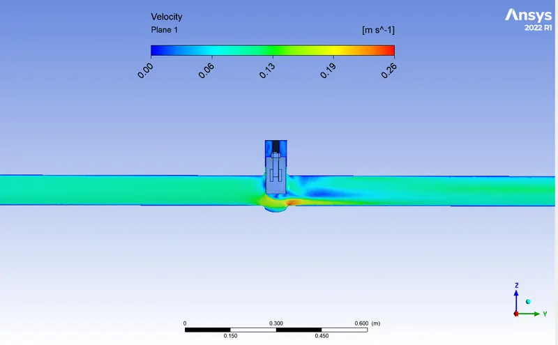
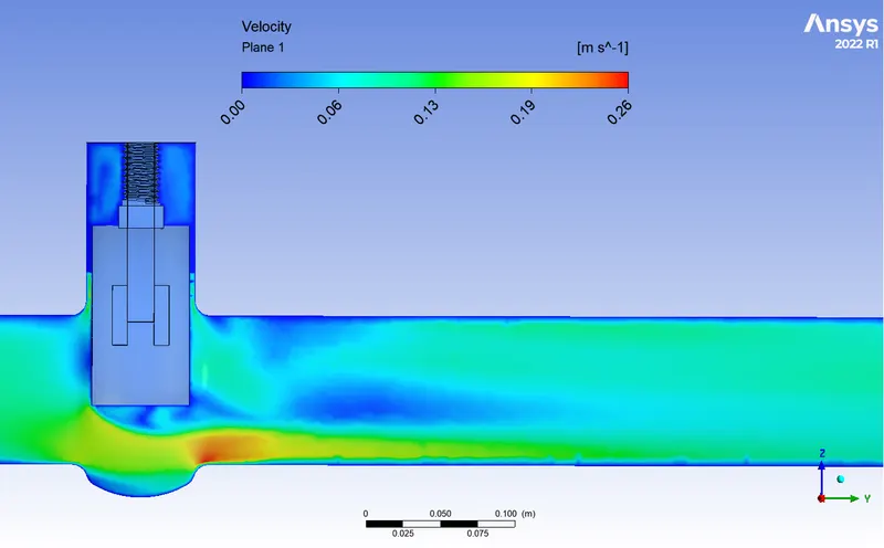
      • The velocity contours represent the variation of the velocity across the direction of the flow.
      • The velocity starts to increase at the opening of the valve and the velocity is maximum at the area shown in red.
      • 
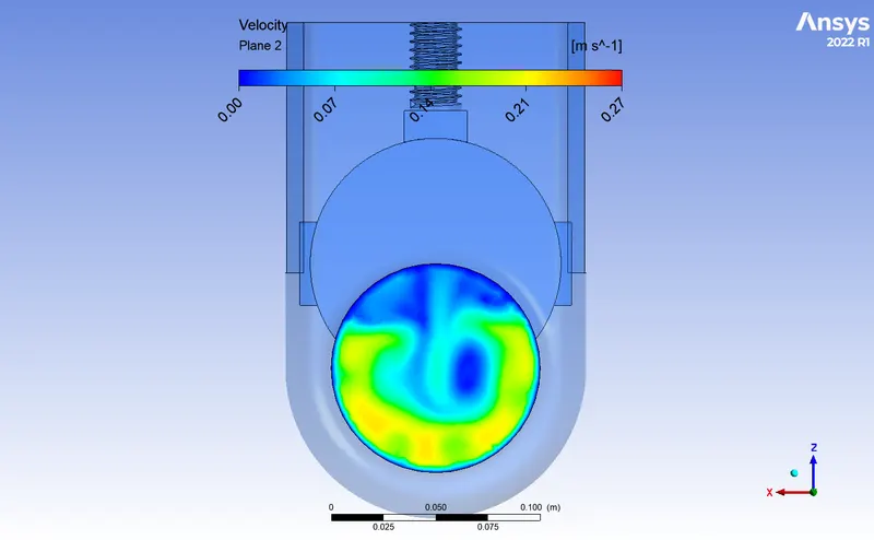
      • This velocity contours of the cross-section of flow shows the pattern of the flow velocity.
      • 
      • 
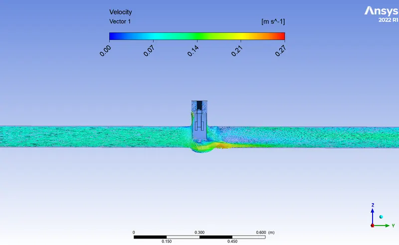
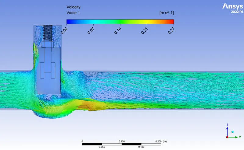
      • The velocity vector plot shows the velocity magnitude and direction of the fluid particles as it can be seen that the fluid particles deflected by the valve gets plunged into the lower bowl part and then at the exit due to the sudden change in the shape of the geometry causes the velocity to increase to the maximum when it gets out of the bowl.
      • THe flow co-efficient for this opening is 260.2 and the flow factor is 225.081.
7. Case-6 (60%):
   1. Openings:
      • 
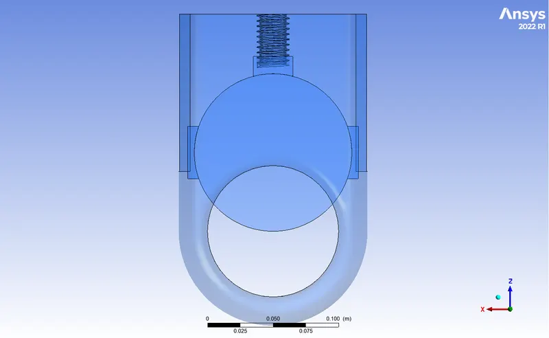
      • The opening of the valve is 60%.
   2. Residuals:
      • 
      • 
      • 
   3. Pressure contours:
      • 
      • 
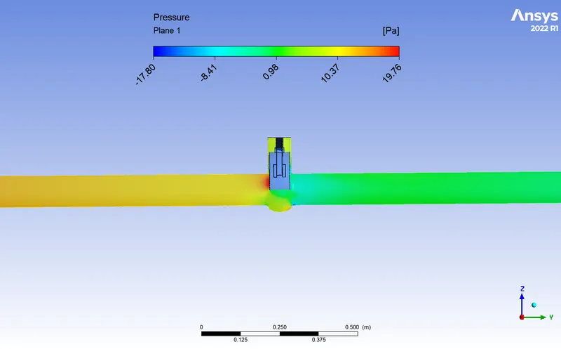
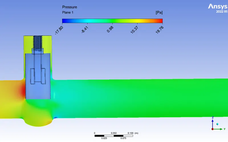
      • The pressure difference at the inlet and the outlet is 13.65 pascals lower than the previous cases.
      • This is attributed to the less restriction caused due to more open valve.
   4. Velocity contours and velocity vectors:
      • 
      • 
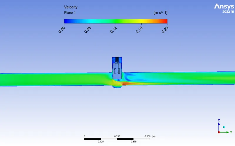
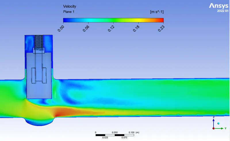
      • The above contour represents the velocity variation of the fluid across the flow.
      • The region marked in red are having highest velocity.
      • 
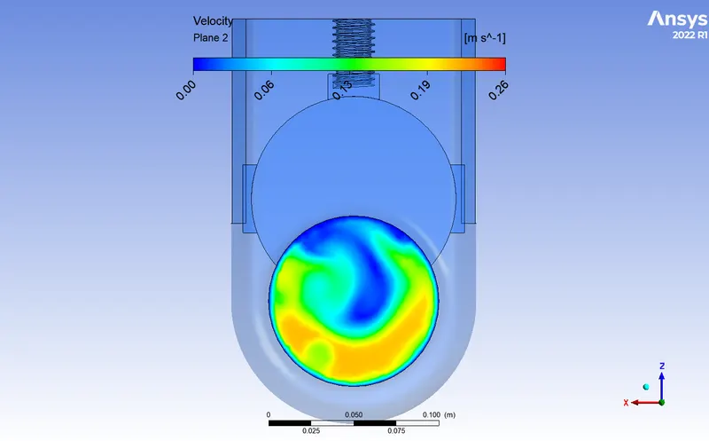
      • The contour represents the velocity variation at the exit of the valve.
      • 
      • 
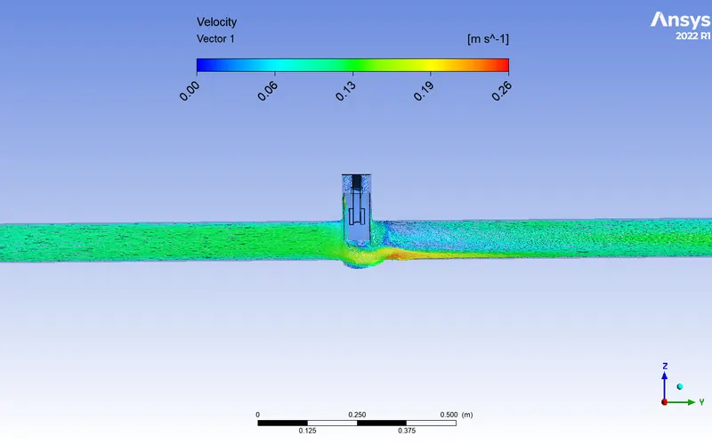
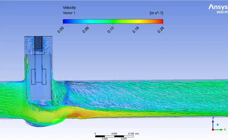
      • The above vector plot represents the velocity vector of the fluid particles across the flow.
      • 
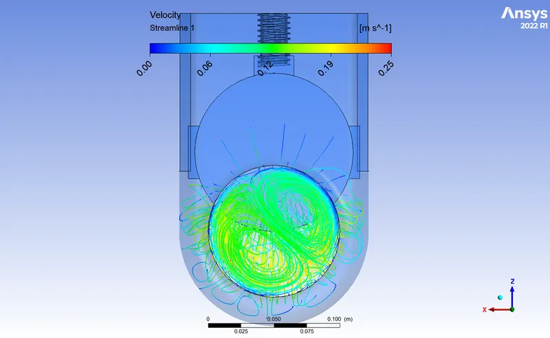
      • The above streamline plot represents the flow pattern and the velocity variation of the fluid particles along the path.
      • It can be clearly seen that at the exit of the valve the fluid forms a circular swirl pattern resulting from the high and low-velocity regions.
      • The flow co-efficient is 313.5 and the flow factor is 271.2.
8. Case-7 (70%):
   1. Openings:
      • 
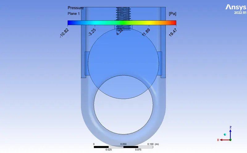
      • Here the opening is 70%.
   2. Residuals:
      • 
      • 
      • 
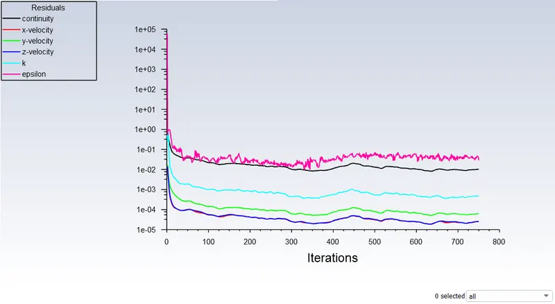
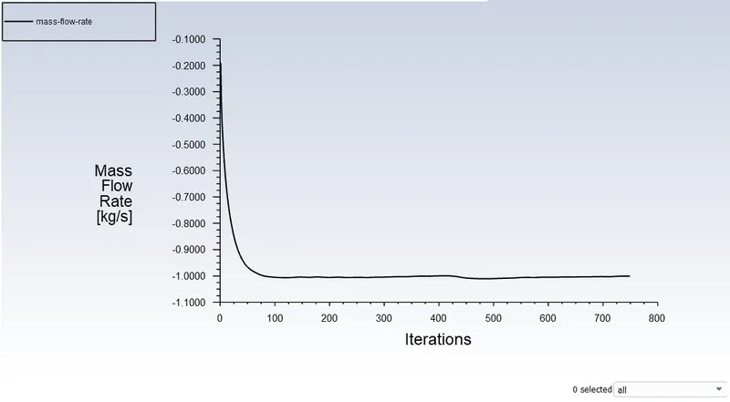
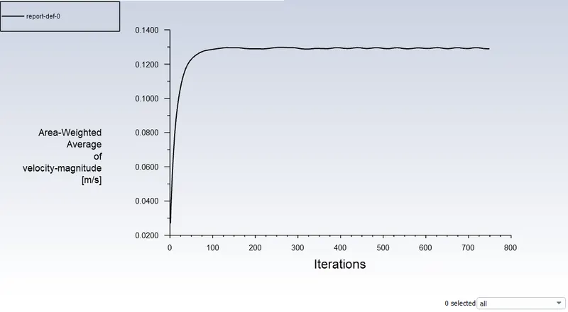
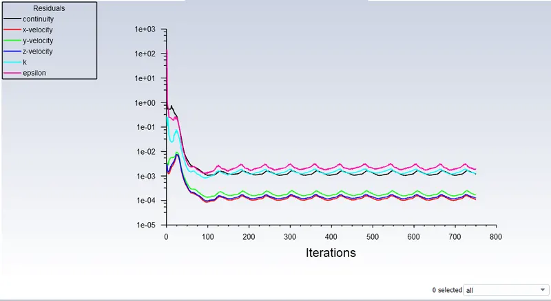
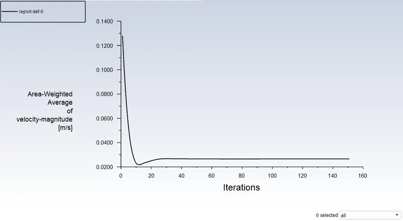
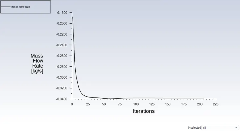
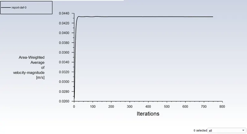
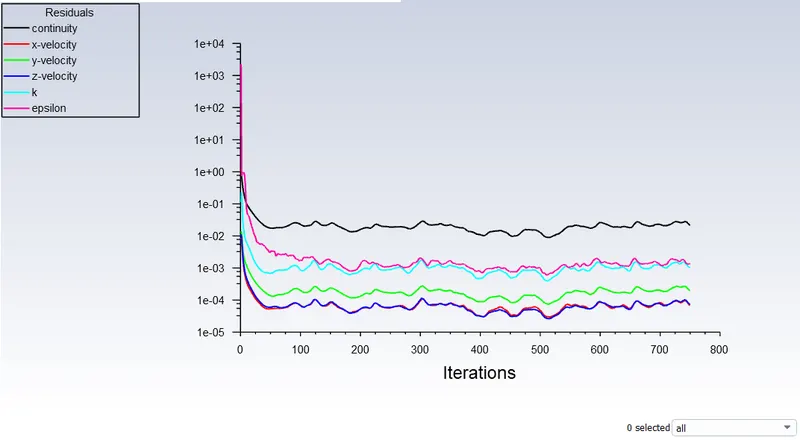
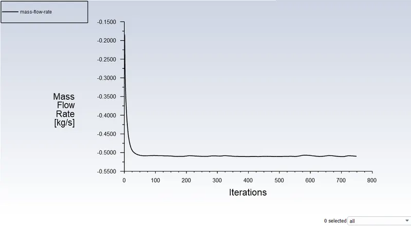
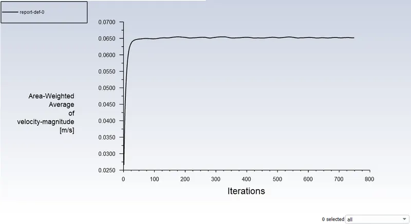
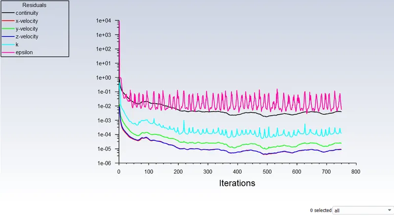
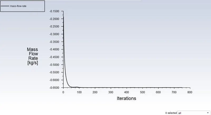
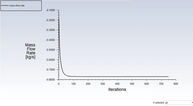
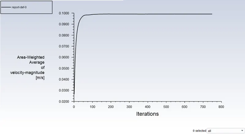
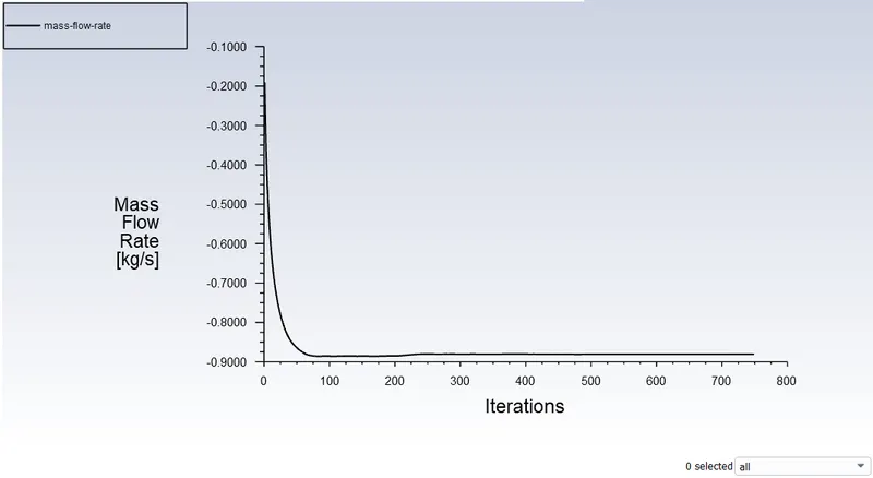
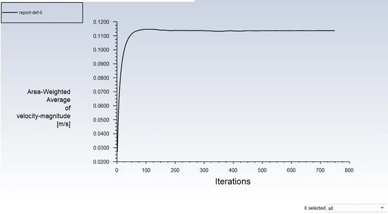
      • The above graphs represent the mass flow rate and the average velocity of the fluid at the outlet and as it has no variations it represents that the convergence is reached.
   3. Pressure contours:
      • 
      • 
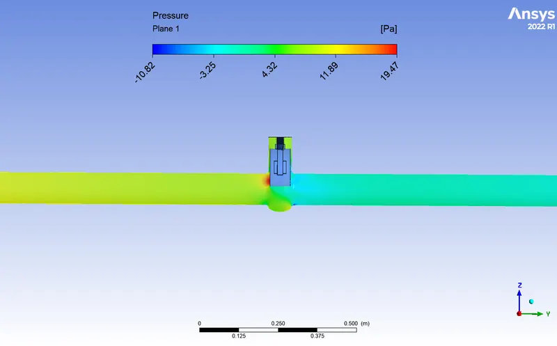
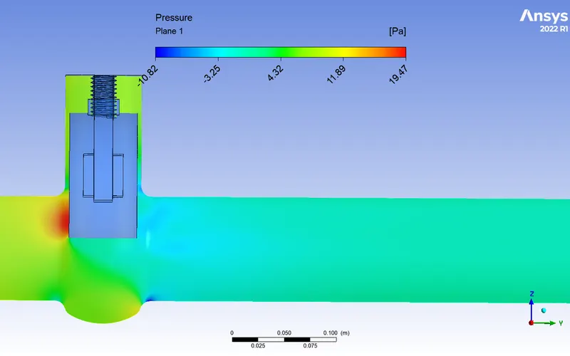
      • The contour represents the pressure variations across the fluid flow path.
      • It can be seen as usual the volume behind the valve has higher pressure due to the obstruction caused by the valve.
      • There is a very high-pressure region marked in red just behind the valve in the upper due to the sudden change in the fluid path caused due to obstruction.
   4. Velocity contours and velocity vectors:
      • 
      • 
      • 
      • 
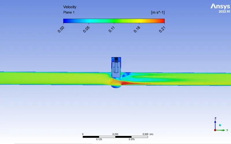
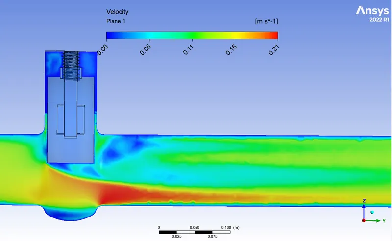
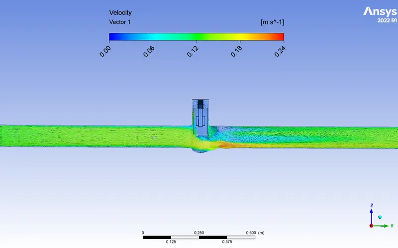
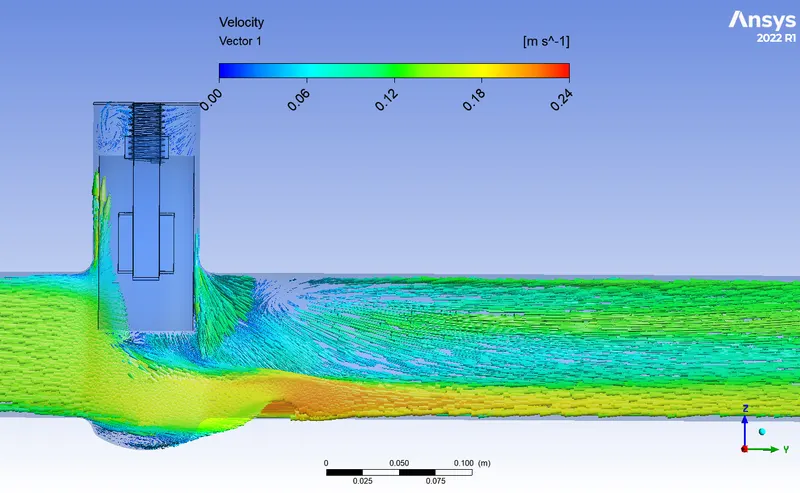
      • The vector plot represents the velocity vector of the fluid particles across the flow.
      • It can be seen that the fluid particles coming out of the valve area have higher velocity.
      • 
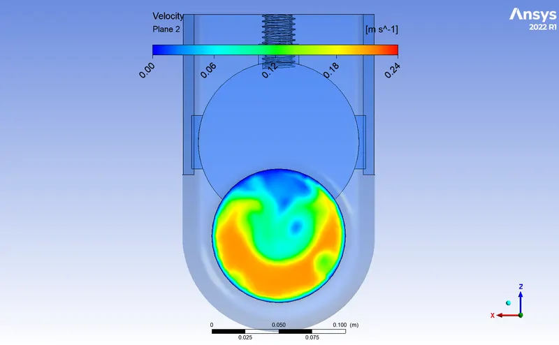
      • The contour represents the velocity profile of the flow.
      • The fluid at the lower region coming out of the valve has high velocity compared to the other region.
      • 
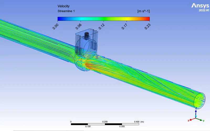
      • This streamline represents the path taken by the fluid particles.
      • 
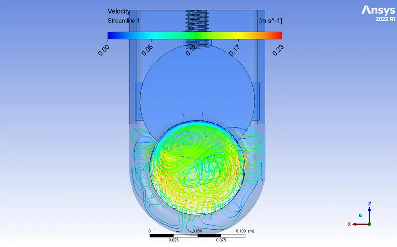
      • The above streamline figure represents the flow pattern and the velocity variation across the flow.
      • The swirls can be seen forming on the top region at the outlet side.
      • The flow co-efficient is 383.36 and the flow factor is 331.6
9. Case-8 (80%):
   1. Openings:
      • 
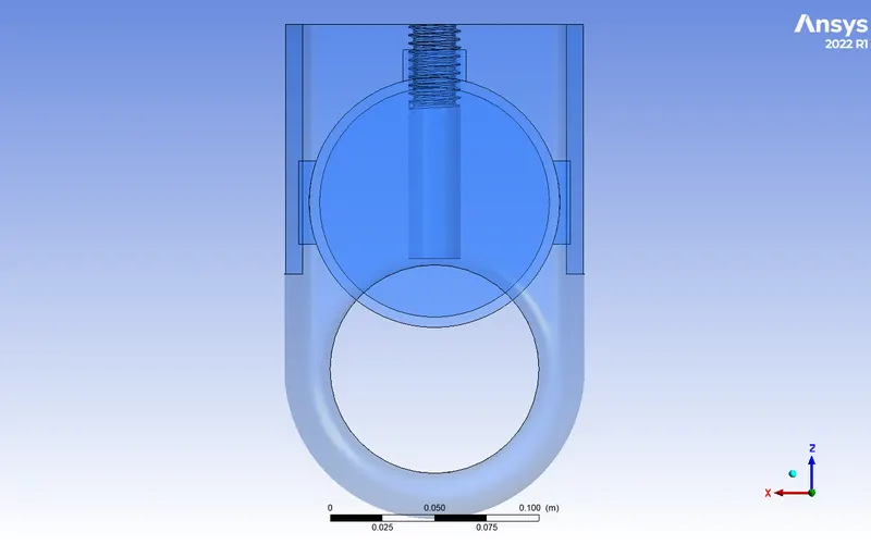
      • Here the valve opening is 80%.
   2. Residuals:
      • 
      • 
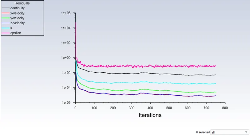
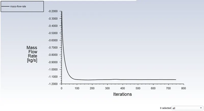
      • The above graph represents the mass flow rate is constant and not changing with respect to the iterations.
   3. Pressure contours:
      • 
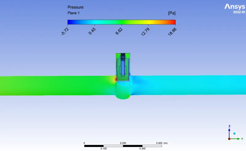
      • The above contour represents the pressure profile across the flow.
      • It shows the high-pressure region at the valve at the inlet side this is due to the obstruction caused due to the valve.
      • The pressure difference is less compared to all the previous cases.
   4. Velocity contours and velocity vectors:
      • 
      • 
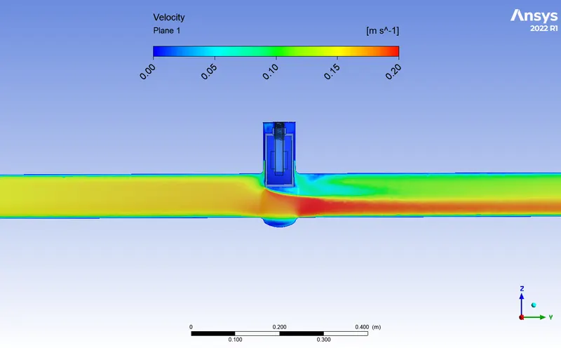
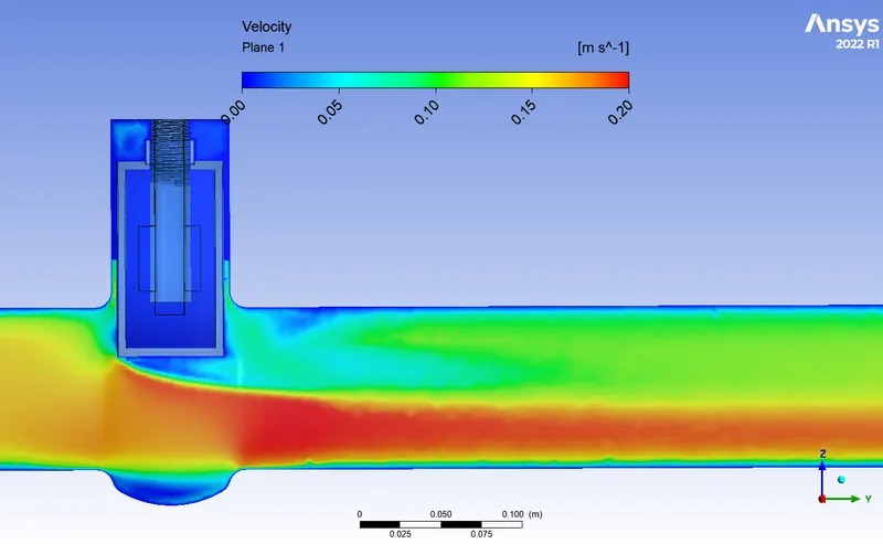
      • The above contours represent the velocity profile across the flow.
      • It can be seen that the fluid particles after exiting the valve have higher velocity and continue in the lower region in the outlet side.
      • 
      • 
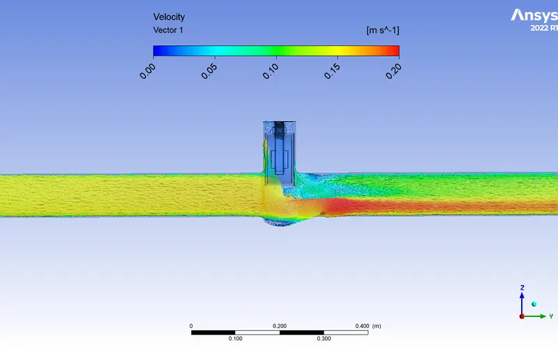
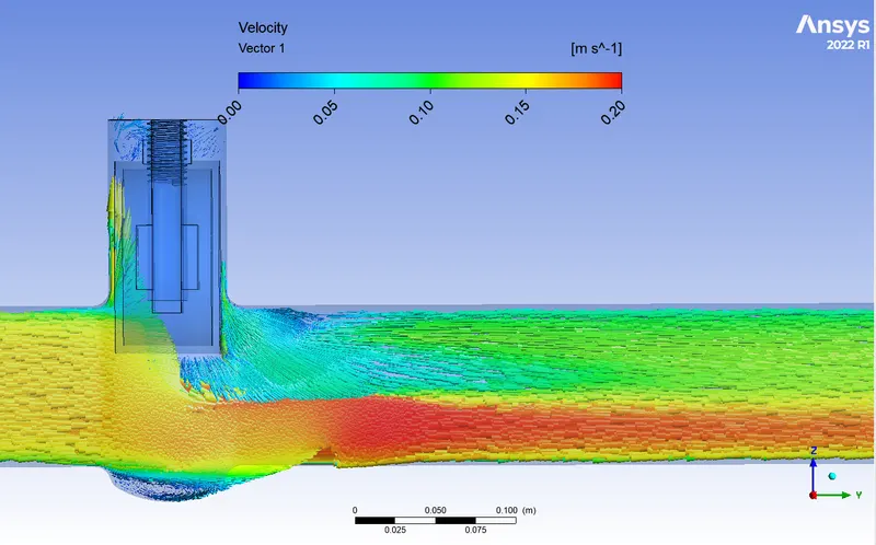
      • The above figure represents the velocity vector of the fluid particles as the flow.
      • It is clear from the vector plot that the fluid in the lower region of the outlet side has more velocity than the upper region.
      • 
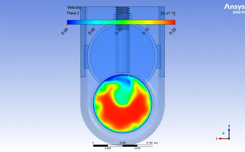
      • It is the contour of the velocity representing the variation of the velocity as it passes the valve.
      • It can be seen that the flow after getting out of the valve forms a swirl and it has higher velocity at the lower region as it comes out of the valve.
      • 
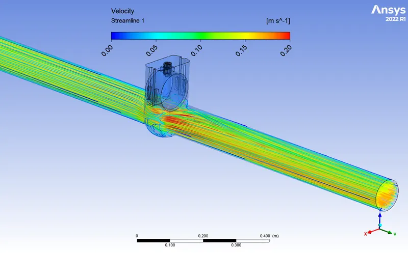
      • The above streamline represents the path taken by the fluid particle as they flow towards the outlet.
      • 
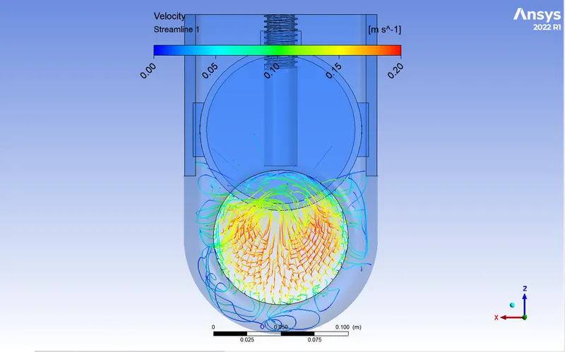
      • The above streamlines represent the flow pattern and the velocity variations in the flow volume.
      • Here it can be seen that the fluid particles after exiting the valve are swirled upwards caused due to the high-velocity region in the lower part and comparatively low-velocity region in the upper part and even due to the fluid particles being pushed out at an angle creating these patterns.
      • The flow co-efficient is 490.89 and the flow factor is 424.62.
10. Table:

    • Open percentage of valve	Mass flow rate (kg/s)		Pressure difference (Pa)			Velocity (m/s)		Flow co-effcient (Cv)			Flow factor (Kv)			Kv To Cv
      	Inlet	Outlet	Inlet	Outlet	Delta	Inlet	Outlet	Pressure (Psi)	Gpm	Cv	Pressure (bar)	VF(m^3/h)	Kv	Kv
      10	0.206248	0.206248	19.65159	0	19.65159	0.026414	0.02654	0.002850122	3.269031	61.233	0.000196516	0.742493	52.966	52.967
      20	0.338375	0.338375	19.06228	0	19.06228	0.043341	0.043364	0.002764653	5.363244	102.002	0.000190623	1.21815	88.229	88.231
      30	0.509764	0.509764	17.87115	0	17.87115	0.065315	0.065334	0.002591899	8.079759	158.705	0.000178711	1.83515	137.276	137.279
      40	0.649496	0.649501	16.54304	0	16.54304	0.083222	0.083346	0.00239928	10.29451	210.167	0.00016543	2.338185	181.791	181.795
      50	0.769597	0.769579	15.15208	0	15.15208	0.098554	0.098855	0.002197546	12.19811	260.210	0.000151521	2.770548	225.076	225.081
      60	0.880470	0.880463	13.65508	0	13.65508	0.112747	0.113164	0.001980433	13.95544	313.591	0.000136551	3.16969	271.250	271.256
      70	1.000657	1.000627	11.80162	0	11.80162	0.128157	0.1284	0.00171162	15.86041	383.364	0.000118016	3.602365	331.602	331.610
      80	1.140714	1.140706	9.353589	0	9.353589	0.146049	0.146149	0.001356576	18.08032	490.890	9.35359E-05	4.106571	424.610	424.620

    • The following table represents the various data like mass flow rate, pressure, velocity, Flow co-efficient(Cv), Flow factor(Kv) etc.
    • These are the values for the individual case of an opening.
    • Gpm represents US gallon per minute.
    • VF (m^3/h) implies a volume flow rate in cubic meters per hour.
11. Flow co-efficient and Flow factor vs opening percentage.
    • 
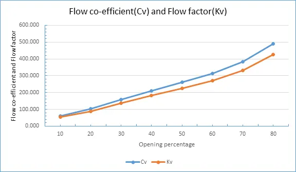
    • The above graph shows the variation of the Flow co-efficient and Flow factor with respect to the opening of the valve.
    • Here it can be clearly seen that the Flow co-efficient and Flow factor increases as the valve is opened and after the 70 percent of valve opening it shows an increase in growth for both flow co-efficient and flow factor
12. Pressure drop vs valve opening:
    • 
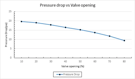
    • The above graph represents the pressure drop variation as the valve is opened.
    • It is very clear from the graph that as the valve opening is increased the pressure difference across the inlet and outlet decreases.

Conclusion:

1. The study is run successfully and the results are analyzed.
2. As the percentage of valve opening increases the pressure difference decreases and velocity increases.
3. The flow patterns and the high-pressure regions are studied and the reasons are analyzed and explained.
4. As the valve opening increases the Flow co-efficient and the Flow factor increases.
5. It can be said that as the valve opening percentage is increased the valve efficiency to allow the fluid flow increases.
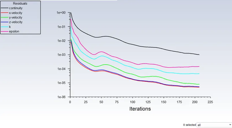
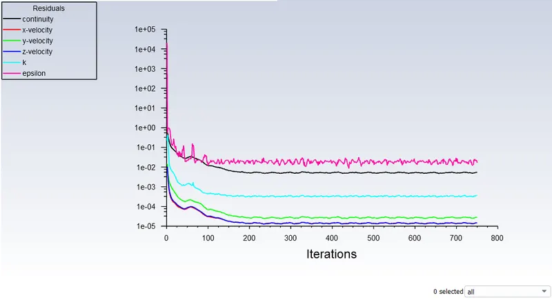
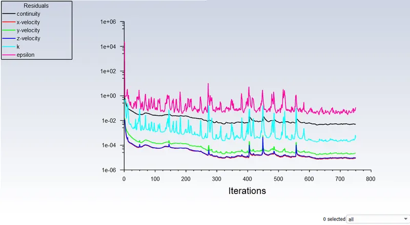
6. The convergence is analysed by residuals, mass flow rate and velocity of the fluid at the outlet.
7. From the convergence plot it is clear that the convergence is achieved as the parameters are not varying with respect o iterations.
8. The study is run for 750 iterations initially then again run for 750 iterations to verify the convergence is achieved and variation is in accordance with the acceptance.
9. The study completed is in accordance with literature available.
10. Note as the opening of the valve increases the mass flow rate increases so where ever the term 'valve opening increases' is stated in the conclusion it also represents the mass flow rate is increasing.

References:

1. Praveen, Jvs. (2017). Flow Coefficient Analysis for a globe valve by using CFD. International Journal of Science and Research (IJSR). 6. 757-763.
2. Nguyen, Quang Khai, Kwang Hyo Jung, Gang Nam Lee, Sung Bu Suh, and Peter To. 2020. "Experimental Study on Pressure Distribution and Flow Coefficient of Globe Valve" Processes 8, no. 7: 875. https://doi.org/10.3390/pr8070875