Week 5 - Rayleigh Taylor Instability

Aim: To perform the Rayleigh Taylor instability simulation for two different fluids and explain the significance and also the difference on the simulation due to grid sizes.

Objectives:

1. Design the fluid regions in the Ansys Spaceclaim.
2. Assign the names to the region.
3. Mesh the geometry.
4. Set the simulation for the VOF(volume of fluid) model.
5. Patch the fluids.
6. Run for the transient time.
7. Note the differences in the simulation due to grid refinement.

Theory:

1. Volume of Fluid (VOF):
   • The volume of fluid method is a surface tracking method for the fluids.
   • This method is useds to calculate the position of the fluid interface which are immisible. 
   • Here the volume fraction of the fluids in each cell are tracked, single momentum equations are shared by the fluis only.
   • These methos are used in:
     1. Stratified flows.
     2. Flow of large bubble in the fluid.
     3. Sloshing effect.
     4. Braking of dam.
     5. Simulations were the position of interface of the fluids needs to tracked/pridicted.
     6. Pridiction if the jet brakeup.
2. Courant Number:
   • It is a dimensionless number which refers to how fast the data is fowing in the descritized domain.
   • The value must be less than 1 so to ensure that the data is within the prescribed elements at the time step.
   • CFL = `U (dt/dx)`
   • CFL<= 1.
   • U = velcoity for the fluid.
   • dt = Difference in time.
   • dx = distance/element length.
3. Rayleigh Taylor Instability:
   • Rayliegh taylor instability (Lord Rayleigh and G.I Taylor) is the instability between the surfaces interfacing of the two fluids which have different densities and were the light fluid is below the heavy fluid resulting in the pushing effect to settle at the top portion of the mixture. 
4. Explicit scheme:
   • It gives the time accurate data.
   • The timestep is crucial as it must satisfy the Courant Number.
5. Implicit scheme:
   • Here the time step need to be varied.
   • It offers the speed of the steady state.
   • Time step is not a constrain.
   • It has superior stability.
   • It is the default scheme in the Ansys fluent.

Content of the body:

1. Open Ansys Spaceclaim and select the sketch plane (xy plane).
   • 
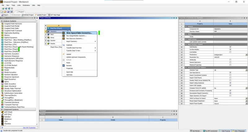
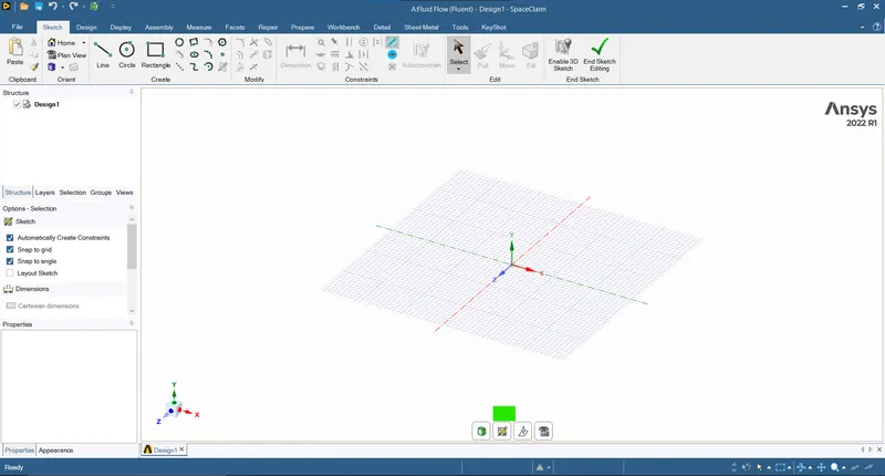
   • Select the sketch plane and the plane on which the geometry modelled:]
   • 
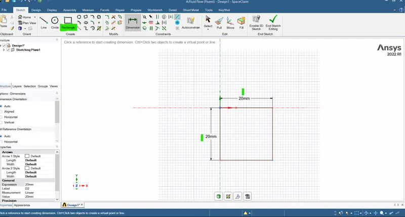
2. Now as the xy plane is selected we can create a rectangle area using the rectangular option in the tab with 20mm width anf 20mm height.
   • 
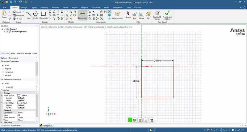
   • Convert to 3D using the 3D option and hit ok:
   • 
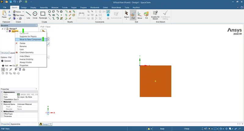
   • Now select the create component option and make this area as a component as there will be base fluid in this part (Design > right click > move to new component > Rename):
   • 
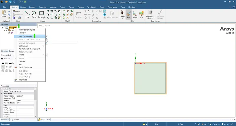
   • Create new surface in same manner above the existing surface and name it as water (Create new component > Create surface > Ok):
   •  
   • 
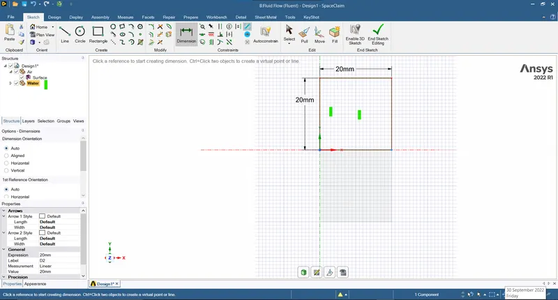
   • Be sure to select the correct component for sketeching.
   • Convert to 3D:
   • 
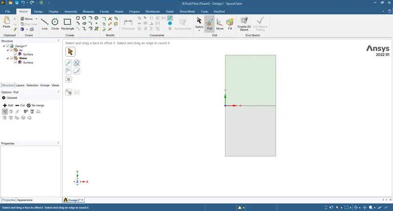
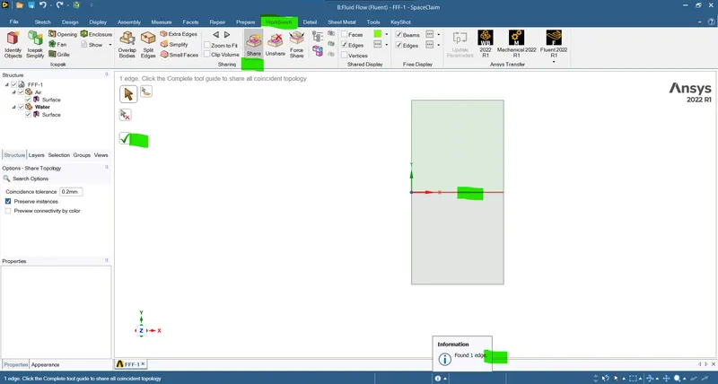
   • Sharing the topology so that the data is shared between the components (Workbench > Share > interfaces > Ok):
   • 
   • 
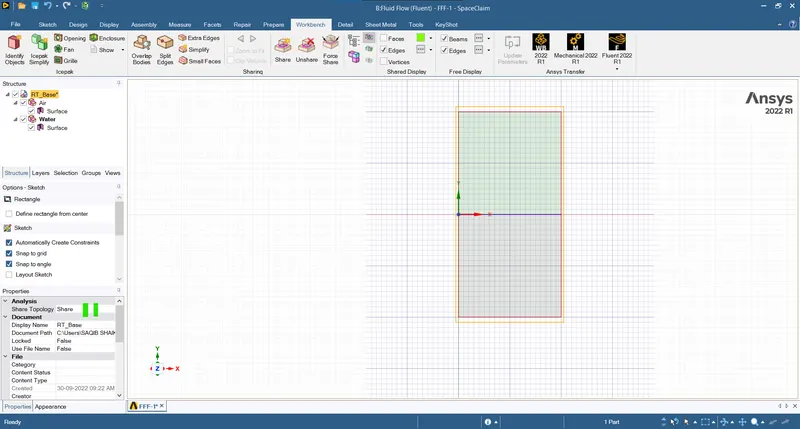
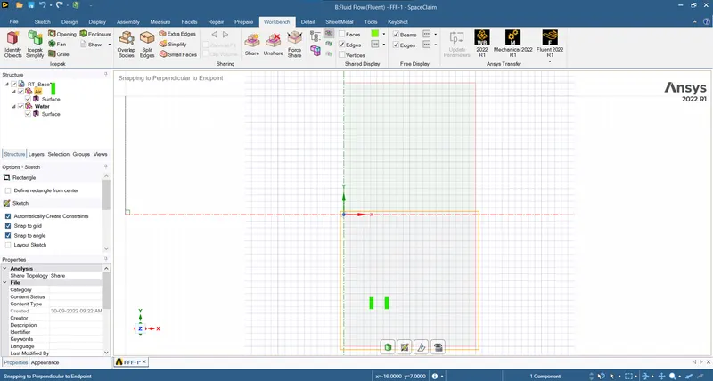
   • Base fluid domain (Air):
   • 
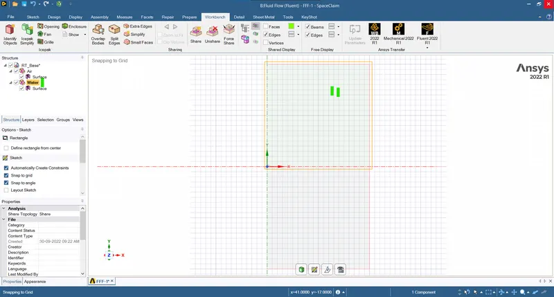
   • Water or user defined domain:
   • 
3. Now as the modelling is complete we can proceed to the meshing.
4. Close the Spaceclaim and open the mesh window in fluent.
   1. 
   2. 
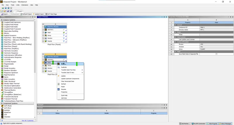
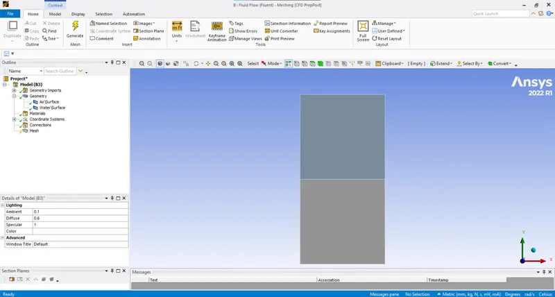
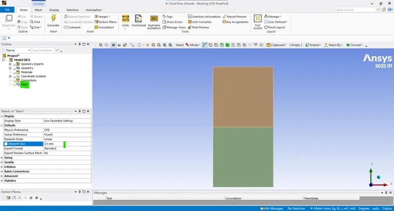
   3. Now defining the mesh element size (Base mesh - 0.5mm):
   4. 
   5. After generating the mesh (Mesh > Right click > Ok):
   6. 
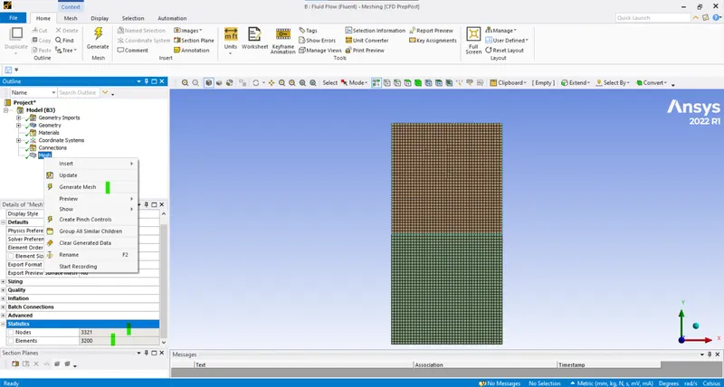
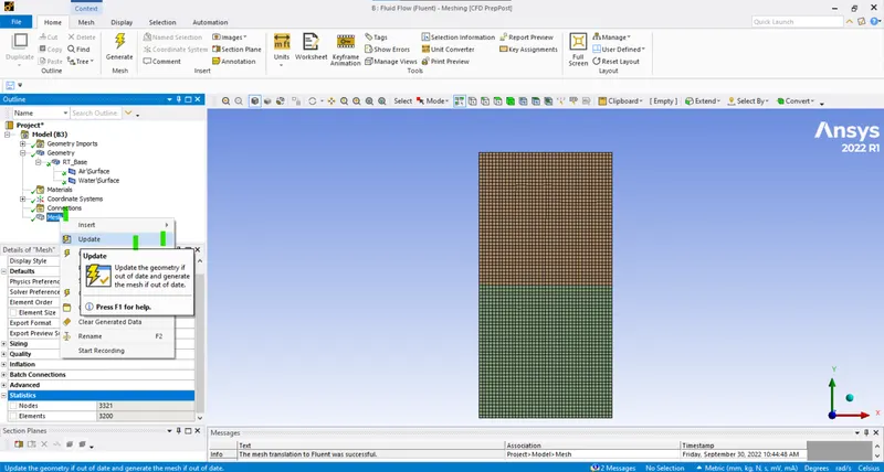
   7. There are 3200 mesh elements.
   8. Update the mesh so the mesh is updated in the directory (Mesh > Right click > Update > Ok).
   9. 
   10. Now the meshing is complete we can move for setting up the physics and conditions.
5. Setup:
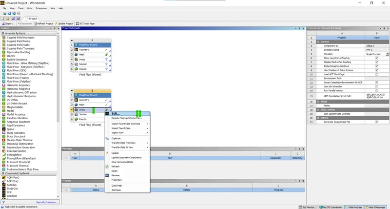
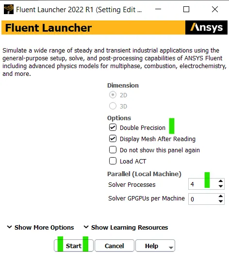
   1. Open the setup window (With double precision):
   2. 
   3. 
   4. Now we are running the simulation in the transient mode with gravity on (in negative y direction - 9.81 m/(sec)^2).
   5. 
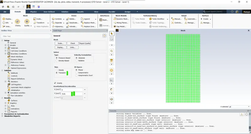
   6. Transient because th state changes with respect to time.
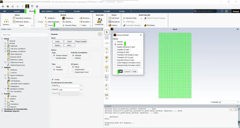
   7. Now selecting the viscous model as laminar flow for the simulation (physics > viscous > Laminar > Ok):
   8. 
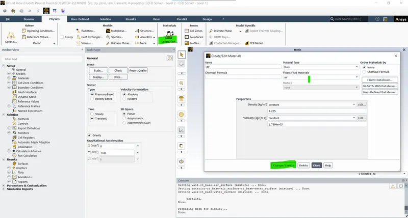
   9. Adding the materials (Physics > Create/Edit materials > Change/Create > Air and water > Ok):
   10. Air:
   11. 
   12. Water (Fluent database > Fluid > Water-liquid > Copy >Ok):
   13. Now opting for multiphase (Physics > Multiphase > VOF > Implicit > Ok):
   14. 
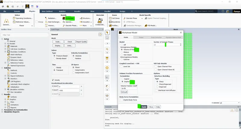
   15. Here as there are two phases so selecting the Eulerian phases as 2.
   16. Here implicit scheme is used beacuse the time step is not assured as the simulation in prelimnary stage, if we use the explicit scheme we need to have the time step in accordance with the courunt number else it will result in floating point error.
   17. Now defining the phases (phases > select the phase with appropriate fluid >Ok):
   18. Here the phase-1 is air (Primary phase):
   19. 
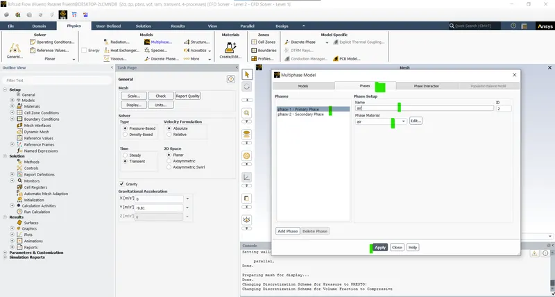
   20. Phase-2 is water liquid (Secondary phase):
   21. 
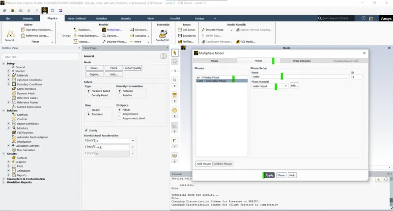
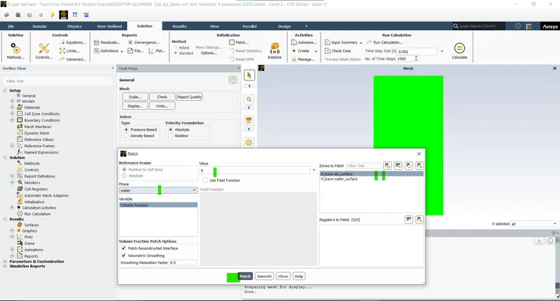
   22. Now patching is done to define the volume fraction of the fluid at the initial time step:
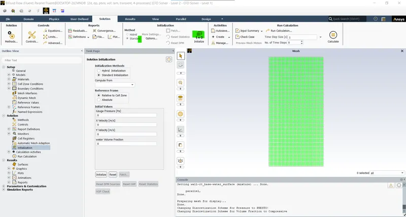
   23. We need to first initialize the setup for this option (Standard Initialization).
   24. 
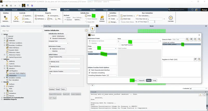
   25. Patch > Water > Volume fraction = 1 > Select the component of water > Patch:
   26. 
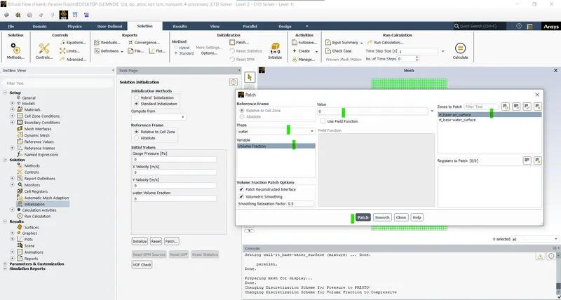
   27. Patch > Water > Volume fraction = 0 > Select the component of air > Patch:
   28. 
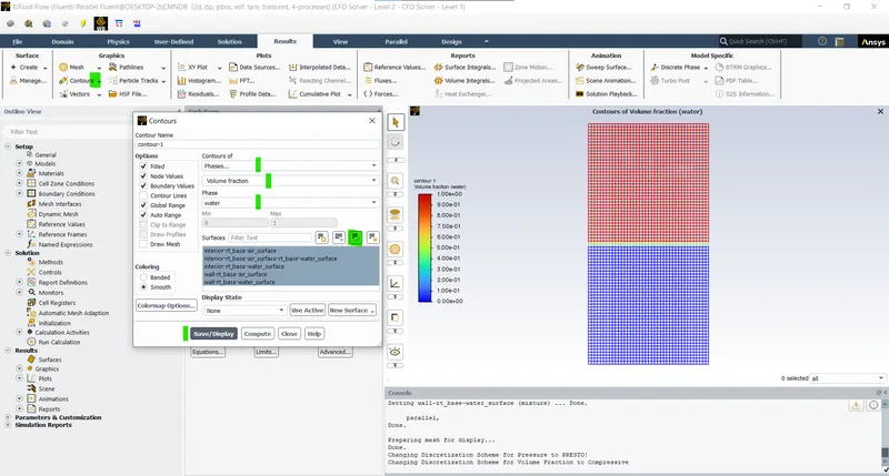
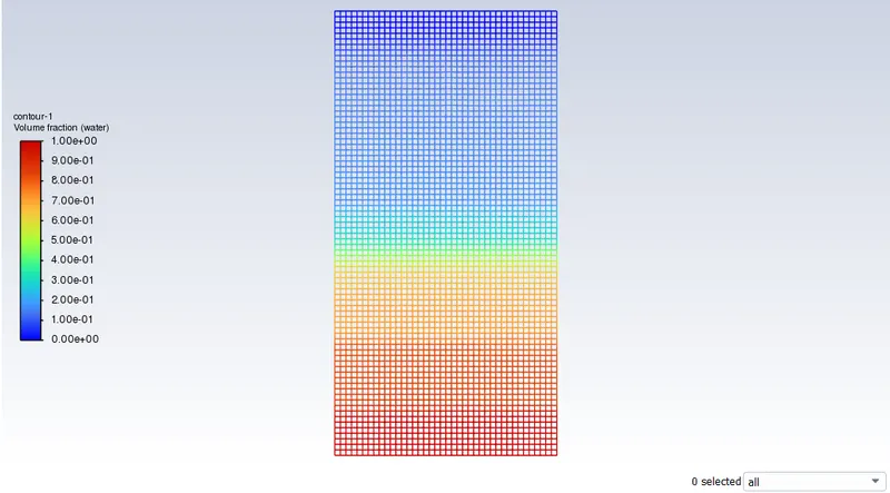
   29. Creating the contours to visualize the effect (Result > Contours > New > Phases > Volume fraction > water > all components > Save and display > Ok):
   30. 
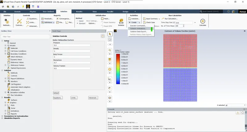
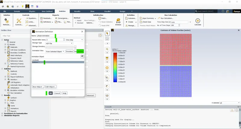
   31. Now creating the animation of the phases motion (Solution animation > Contours > Phases > Ok):
   32. 
   33. 
   34. Now run the simulation for 500 time step with 0.01 as time step:
   35. 
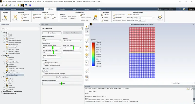
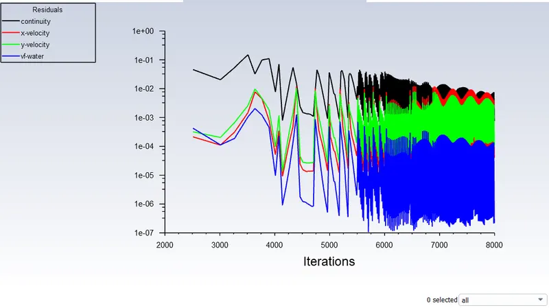
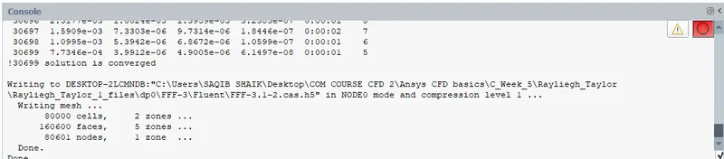
   36. The solution is converged at 7996 iteration, 4.99 seconds.
   37. Residuals:
   38. 
   39. Phase contours:
   40. 
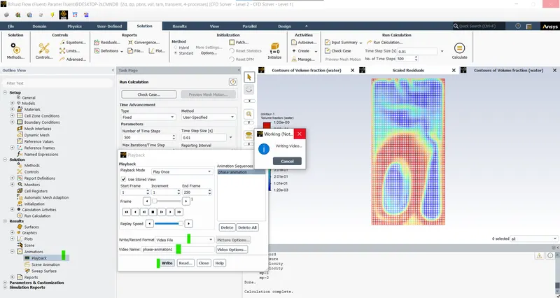
   41. Save the animation file as Results > Animations > Play back > Video file > enter the name > ok.
   42. 
   43. 
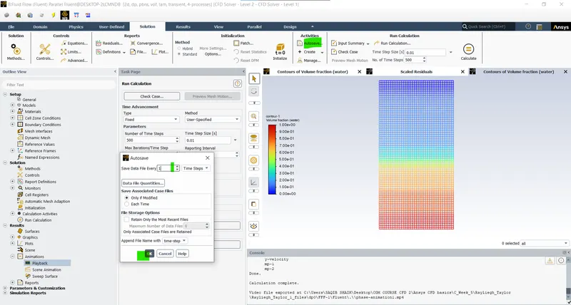
   44. There is another method to extract the animation in the post processor, to to that we need to save the data at defined time step (Auto save > define the frequency of data to be saved > Ok):
   45. 
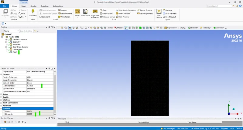
   46. Now running the second case with refined mesh (Element size - 0.1mm - 80,000 elements)
   47. 
   48. Case-3, here the air is replaced with the fluid with userdefined properties:
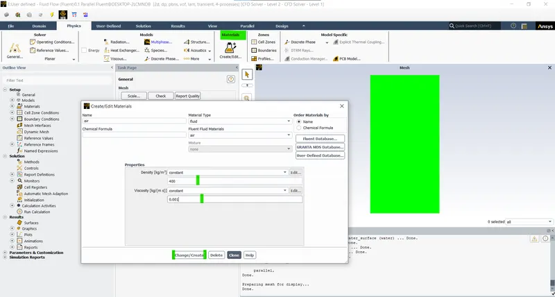
   49. Properties of the userdefined fluid:
       1. Density = 400 kg/m³,
       2. Viscosity = 0.001 kg/m-s
   50. Change the properties in the materials tab (Materials > Change the values > Rename > Change create):
   51. 
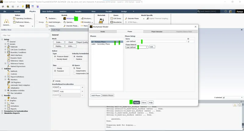
   52. Change the primary phase as user defined fluid (Multiphase > Phase > Primary Phase > Select respective phase > Apply):
   53. 
   54. Initialize and patch the volume fraction:
   55. Water volume fraction in water component = 1:
   56. 
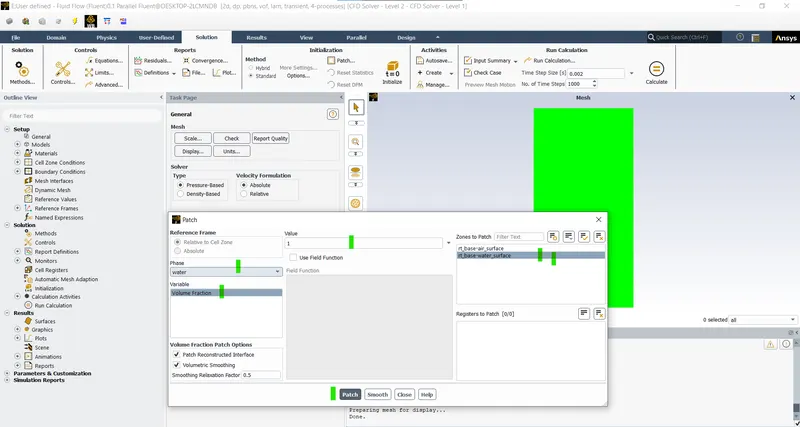
   57. Water in air/userdefined component = 0:
   58. 
   59. Running the simualtions with the time steps as mentioned below:

   60. Cases	Time step	Number of steps	Total time period
       1	0.01	500	5    sec
       2	0.002	1100	2.2 sec
       	0.004	700	5.2 sec
       3	0.002	1500	3    sec
       	0.004	200	3.8 sec
       	0.005	100	4.3 sec
       	0.006	50	4.6 sec

Results:

Case-1 (Basic Mesh):

1. Residuals:
   • 
2. Phase contours:
   • 

Case-2 (Refined water and air):

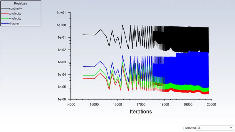
1. Residuals:(2 secs)
   • 
2. Phase contours:
   • 2 seconds
   • 
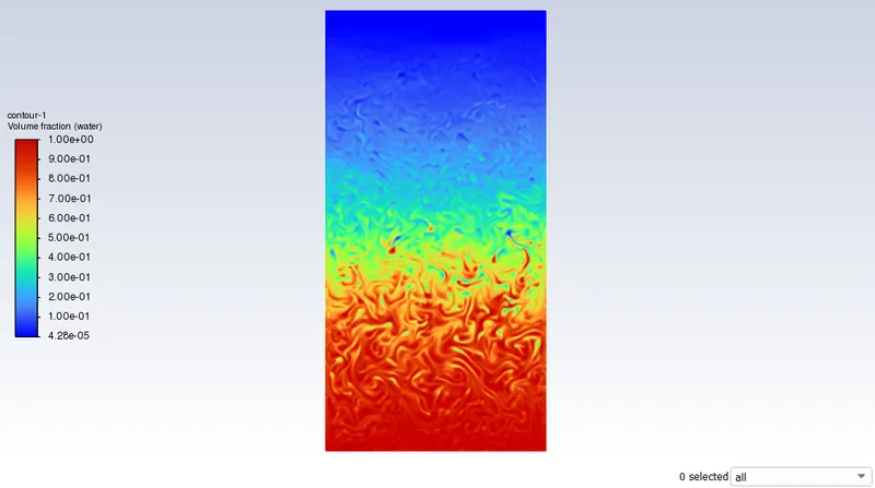
   • 4.18 seconds
   • 
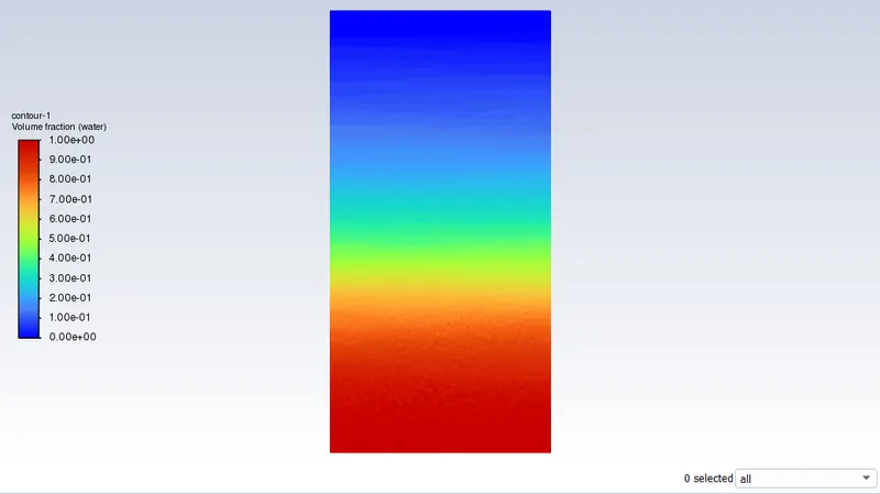
3. Convergence:
   • 

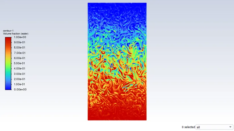
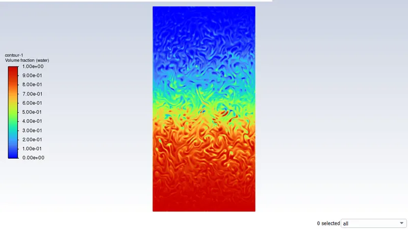
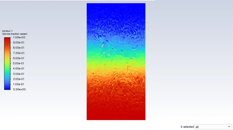
Case-3: Refined and userdefined.

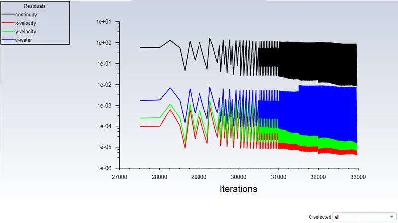
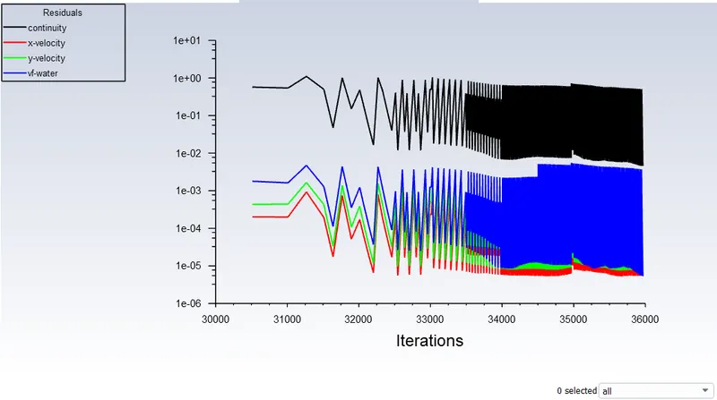
1. Reisduals:
   • 3 seconds (0.002*1500)
   • 
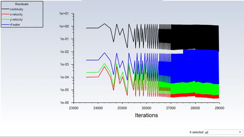
   • 3.8 seconds (0.004*200) + 4.3 seconds (0.005*100):
   • 
   • 4.6 seconds (0.006*50):
   • 
2. Phase contours:
   • 3 seconds (0.002*1500)
   • 
   • 3.8 seconds (0.004*200) + 4.3 seconds (0.005*100):
   • 
   • 4.6 seconds (0.006*50):
   • 
3. Contents summary table:

   • Cases	Time step	Number of steps	Total time period	Animations
     1	0.01	500	5.0 sec	Case-1 (Water-Air)
     2	0.002	1100	2.2 sec	Case-2 (Water-Air-Refined)
     	0.004	700	5.2 sec
     3	0.002	1500	3.0 sec	Case-3 (Water-User defined-Refined) Case-3 (Water-User defined-Refined) Case-3 (Water-User defined-Refined)
     	0.004	200	3.8 sec
     	0.005	100	4.3 sec
     	0.006	50	4.6 sec

1. What are some practical CFD models that have been based on the mathematical analysis of Rayleigh Taylor waves? In your own words, explain how these mathematical models have been adapted for CFD calculations.
   • Some practical CFD models based on the mathematical analysis of Rayleigh Taylor waves are:
   • Plateau-Rayleigh instability:
     • This model is often also known known as Rayleigh instability it is used to study/simulate the fluid stream falling and dispersing into smaller segments.
     • Here main point when the fluid falls and dispers its volume remains same but the surface area changes.
     • This is useful in many simulation to assess the behaviour of the stream falling, dispersing and settling.
     • Major application includes specfic types of the inkjet technology.
     • It can also be used in the studing the droplets from the injector.
   • Richtmyer–Meshkov instability (RMI):
     • This model is used to simulate the instability occurs when the two fluids of different density are suddenly/impulsively accelerated.
     • Generally this model is used to simulate the shock wave interaction with the fluids.
     • This model is considered as the impulsive-acceleration limit for the Rayleigh Taylor instability.
     • Here the shock is considered as the impulsive compression which propagates non linearly and transitions to the turbulent behaviour. 
   • Kelvin–Helmholtz instability:
     • This instability model is used for the study/simulation of the fluids consisting of the  velocity shear.
     • The instability occurs when there is a velocity shear between the strata of the same fluid and/or at the interface of the two fluid surface.
     • The applications include the wind flowing over the water surface, cloud formations, smoke exiting the chimney, air circulators and even the atmosphere of the sun.
2. Explain why a steady-state approach might not be suitable for these types of simulation.
   • Steady state simulation are best suited for the cases were the end results are of greater concerns but as in the current case the change in state is completely time dependent as we need to observe the changes in the states as the time proceeds tom study the interactions between the surfaces which can't be studied in the steady state solver more accuratly as the steady state simulations do not produce time accurate data.
   • So here the transient state solver is used as we are more concerned about the stages of the interaction with respect to time (we need time accurate data) which in the steady state solver is immposible to assess, so for the cases were the intermediatery states are very important with time accuate data transient state solver must be used.
3. Define the Atwood Number. Find out the Atwood number for both the cases and explain how the variation in Atwood number in the above two cases affects the behavior of the instability. 
   • Atwood number is a dimensionless number used in fluid dynamics to study the hydrodynamic instabilities in the density strtified fluids.
   • In the Rayleigh taylor insability the Atwood number is useful in studying the heaviour fluid bubbles penetration distance into the less denser fluid which is the function of acceleration and time.
   • Its formula representing as:
   •  `Atwo od Number = (rho_1-rho_2)/(rho_1+rho_2)`
   • `rho_1 = density-of-heavy-fluid`
   • `rho_2 = density-of-lighter-fluid`
4. Atwood number:
   1. For case-1(Water-Air):
      • Density of air = 1.225 `(kg)/m^3`
      • Density of water = 998.2 `(kg)/m^3`
      • Atwood number = `(998.2-1.225)/(998.2+1.225)` = 0.9975
   2. For case-3 (Water-User defined fluid):
      • Density of User defined fluid = 400  `(kg)/m^3`
      • Density of water = 998.2 `(kg)/m^3`
      • Atwood number = `(998.2-400)/(998.2+400)` = 0.42783
   3. In the present cases when we have a higher Atwood number meaning the density difference is large we will be have a very voilent mixing which will in turn results in the best type of mixing with the given time and they will take less time to settle as per there densities, and when the Atwood number is low meaning the density difference is less in this case the mixing will be comparetively slow and it will take more time to reach to saturate conditions and we see more patterns as the both fluids try to settle as per there densities, the Atwood number also helps in study of how deep the heavey fluid instantly move in the less denser fluid at the start i.e. if the Atwood number is high the heavy fluid penetrates more distance in the lighter fluid as compared to the mixture with less Atwood number.

Conclusions:

1. The simulation is run successfully run for the given cases.
2. The mesh refinement has a very major impact on the simulation results specially the animation and the settling time accuracy.
3. As the mesh is refined the we can observe the fluid interface interactions very accuratly and the settling time can be predicted more accuratly as the mesh is more refined (provides more resolution).
4. The solution results are dissucused and documented.
5. The difference between the surface interaction with the fluids with different densities can be observed very clearly.
6. We can see from the simulation that when the difference in the density is more the fluids settles in comparetively to the fluids having less difference in the densities.
7. The behavior of the motion of fluids during the settling also is very different as the mixture with less density difference have more swirls and vortex forming during the settling process.