Week 1- Mixing Tee
Aim: To perform the simulation on the mixing tee for the thermal analysis and study the effect of the length and momentum ratio on the mixing effectiveness of the mixing tee.
Objective of the project:
- Importing the geometry in the Ansys Fluid Flow Fluent.
- Extracting the fluid volume which is under study.
- Meshing the geometry.
- Perform the grid independent study.
- Set the boundary conditions.
- Compare and select the k-epsilon and k-omega SST model.
- And solve using the most useful model in the solver (k-epsilon and k-omega SST) stating the reasons.
- Compare the results for different momentum ratio and lengths.
Theory:
- The thermal analysis helps use to simulate the thermal parameters of the case in study, which points out the bottleneck issues/conditions, factors effecting the output parameters and unwanted developments, which will intern helps in better development/iteration of the product.
- The theoretical temperature at the outlet is calculated by using the formula extracted from the balancing equations:
- Tmix = `((m_(hot) * T_(hot) )+(m_(cold) * T_(cold)))/(m_(hot)+m_(cold)`
- were
- mhot = mass of hot fluid fluid (kg/s).
- mcold = mass of cold fluid (kg/s).
- Tcold = Temperature of cold (c).
- Thot = Temperature of hot (c).
- Tmix = Temperature at the outlet after mixing.
Content of the body:
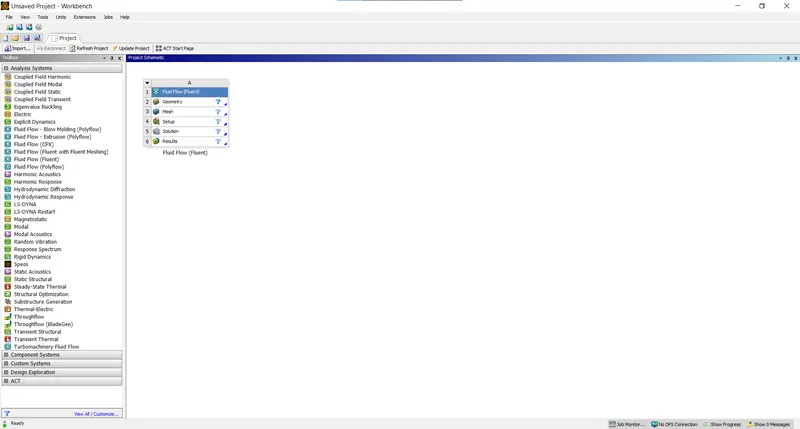
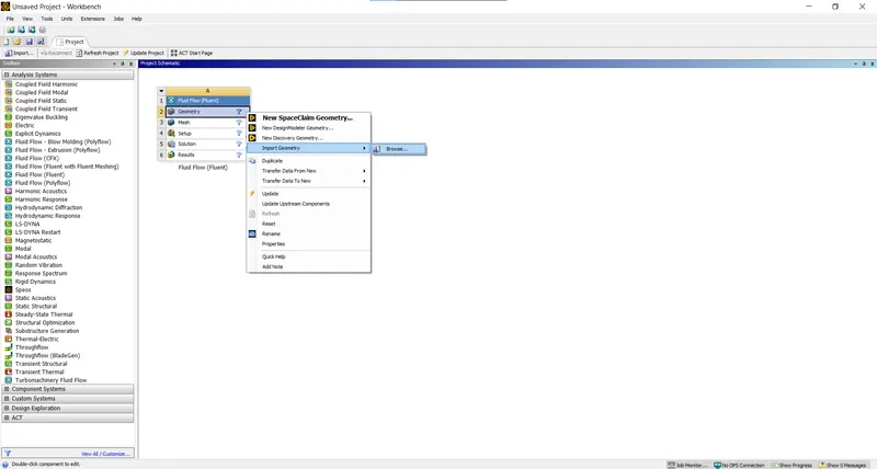
- Open the Ansys workbench and Fluid Flow (Fluent):
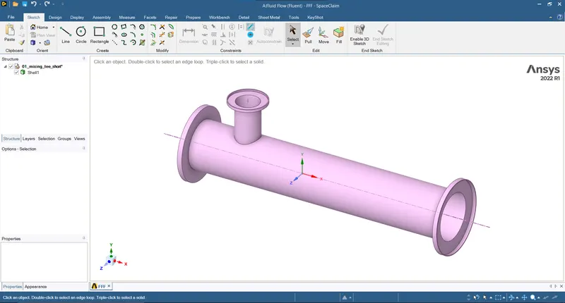
- Now import the geometry either in geometry option(Right Click > Import):
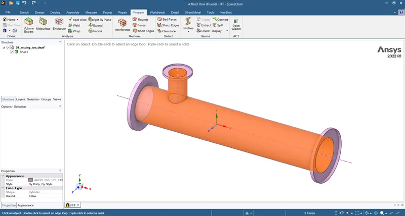
- Using the Volume Extract option in the Prepare tab extract the inner volume and supress the outer body for the physics as it doesn't have any function(not a conjugate heat transfer problem):
- The geometry shown is only the fluid volume which is needed for the analysis:
- Using the select edges options:
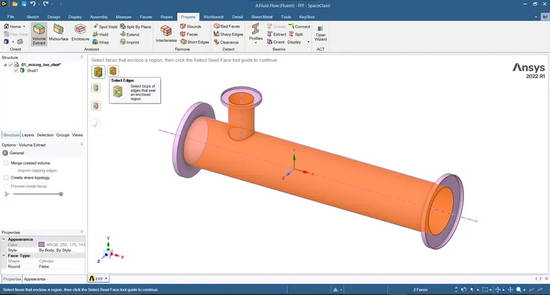
- Select all the three options:
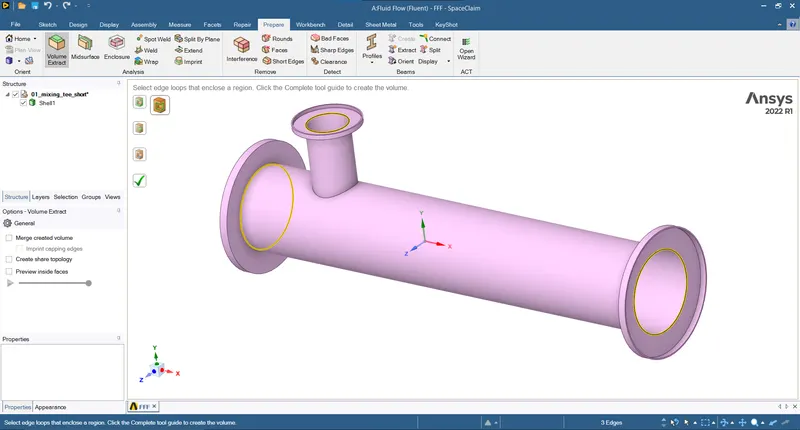
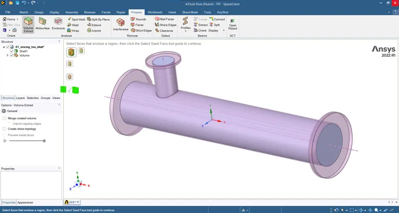
- The geometry shown is only the fluid volume which is needed for the analysis:
- A new volume is created and the outter solid shell is suppressed by option suppress for physics in the Structure tab:
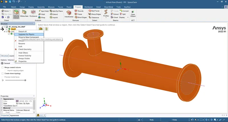
- Outter body is Supressed and hidden:
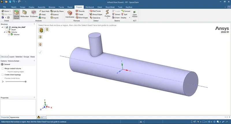
- Now the gemetry part of the simulation is completed, close the Ansys space claim.
- Meshing:
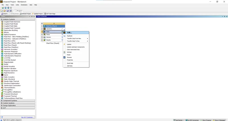
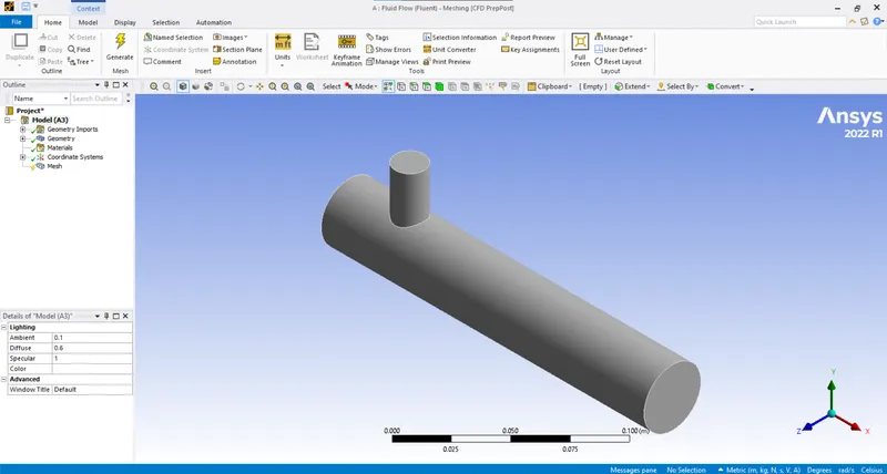
- Now open the mixing tee in the meshing environment(Mesh > Edit > ok):
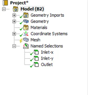
- Here the meshing and naming of the inlet and outle ports are performed.
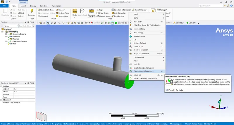
- Naming the openings (select face > Right click > Create named selections):
- Inlet-x or Hot_Inlet:
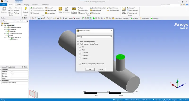
- Inlet-y or Cold_Inlet:
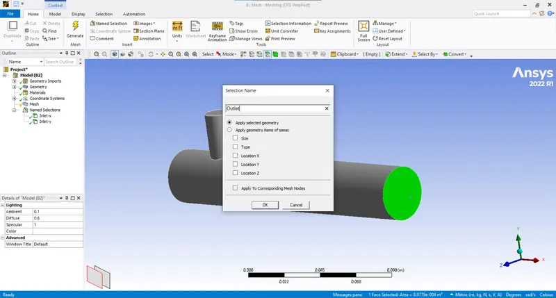
- Outlet:
- Inlet-x or Hot_Inlet:
- For the meshing first the mesh independency should be the main concern.
- For the mesh independency test we are considering three cases:
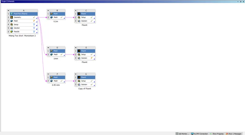
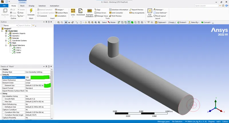
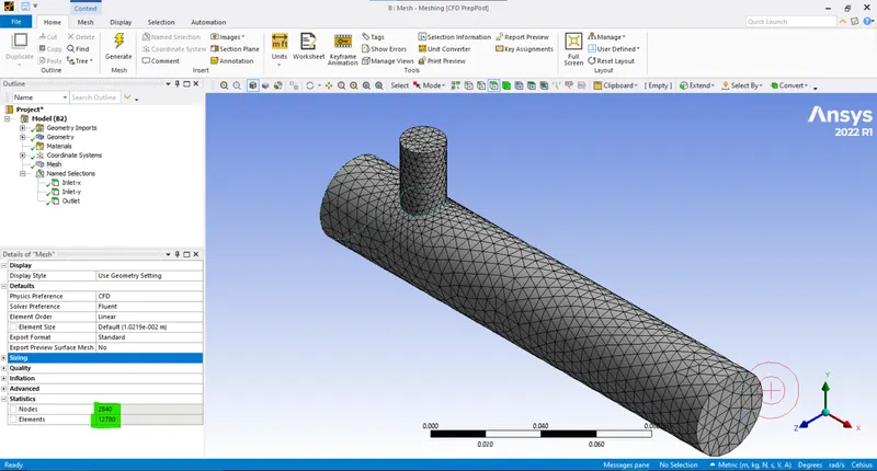
- With default mesh settings(Element size - 0.01 meter):
- Change the physics reference to CFD:
- Generate mesh (mesh > Generate mesh):
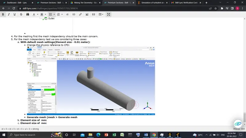
- As it can be seen it has very course mesh with the 12780 elements:
- Setting up boundary conditions for the model with slected values and comparing.
- Element size of 1 mm:
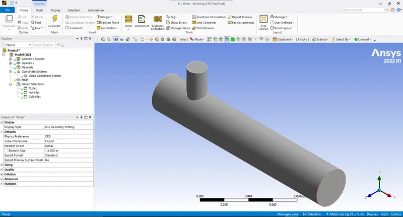
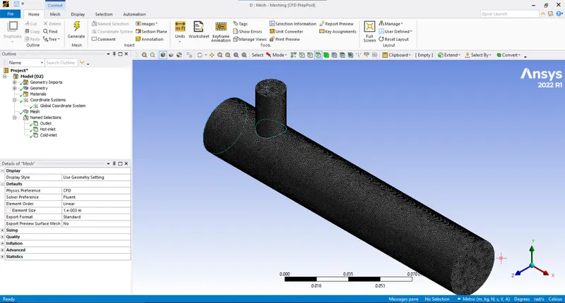
- Total number of mesh elements are 576721.
- Element size of 0.95mm:
- Total number of mesh elements are 743463
- Grid Independency:
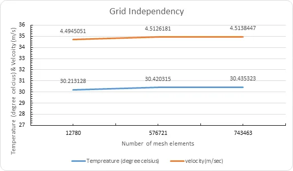
- It is observed that there is no significant effect on the results after 1 mm element length (576721 elements) so, it can be considered as the Independent mesh size.
- As we observe there in no significant effect of the number of mesh elements on the solution we can proceed with the 1mm element length.
- Now select the mesh option and generate the mesh (Mesh > Right click > Generate mesh > Ok):
- Now creating the Inflation layers for more accurate visualization:
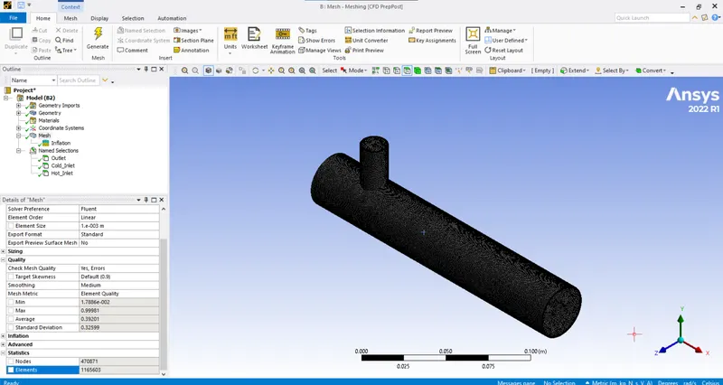
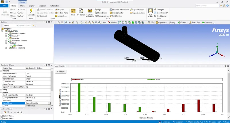
- Viewing the mesh matrics data of the mesh elements:
- Using the section plane option to view the section of the geometry:
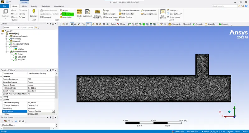
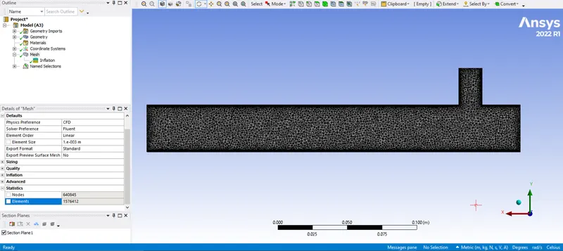
- Now the mesh elements is 1165603 for short tee (For long tee - 1576412).
- As we have enountered some issues the new mesh without inflation layer is done and the calculation are rerun(explained in results):
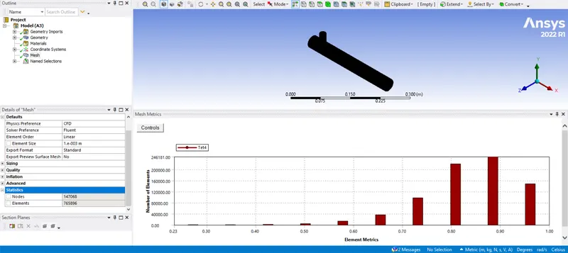
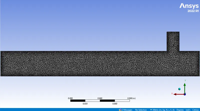
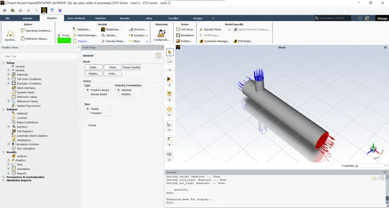
- The mesh is generated and ready to setup in the solver.
- Setup:
- Using the double precision for the solver setup and parallel cores:
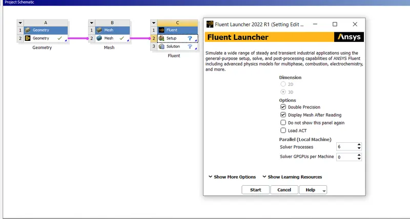
- Double precision is used to represent each floating point number using the 64 bits
- We are solving the problem in the pressure based solver (Fluid velocity less than mach 3) with steady state conditions:
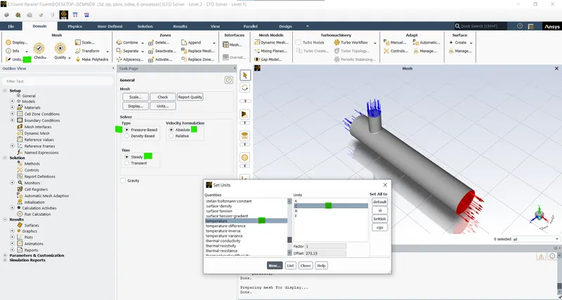
- And Units option from the tools bar is used to change any requried units of the parameters.
- As we are simulating the temperatures we need to activate the 'Energy Equation' for the solver in the Physics tab:
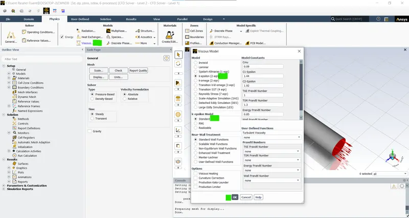
- Now viscous model is selected for the turbulent flow:
- Here the k-epsilon model is selected for the viscous model (explained below) (Viscous model > k-epsilon > Std > Ok):
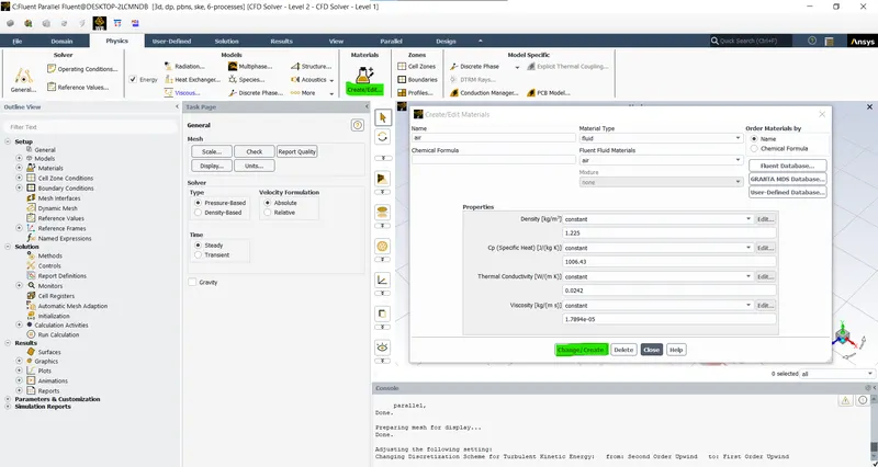
- Adding the fluids used in the library (Materials > Create/Edit > Select Fluid > Air > Change/Create):
- Defining the Working Fluid:
- Since the fluid is working only in the volume so defining it will be enough (Cell Zones > Select Volume > Edit > Material Name > Working Fluid > Apply) :
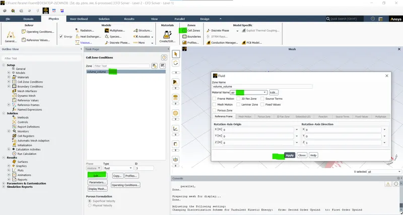
- Defining the Boundary Conditions:
- Defining the inlet type and outlet type if not automatically selected by the fluent solver:
- Defining the inlet as velocity inlet and defining the velocity and temperature:
- Short Tee:
- Momentum Ratio = 2:
- Cold Fluid Inlet:
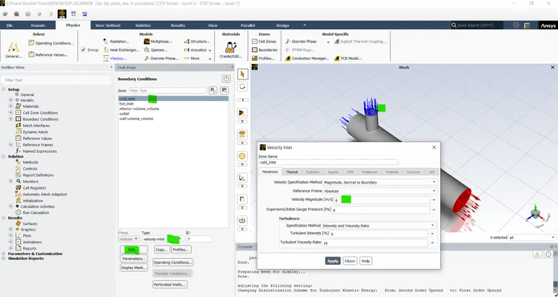
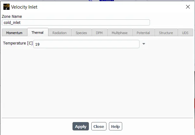
- Momentum Ratio = Cold Fluid velocity / Hot Fluid Velocity
- Cold Fluid Velocity = 6 m/s.
- Temperature = 19 degree celsius
- Hot Fluid Inlet:
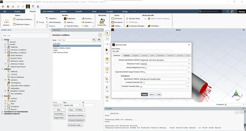
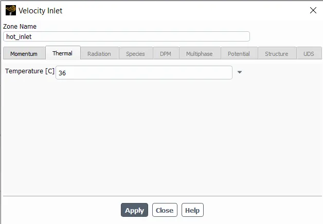
- Hot Inlet Velocity = 3 m/s
- Temperature = 36 degree celsius
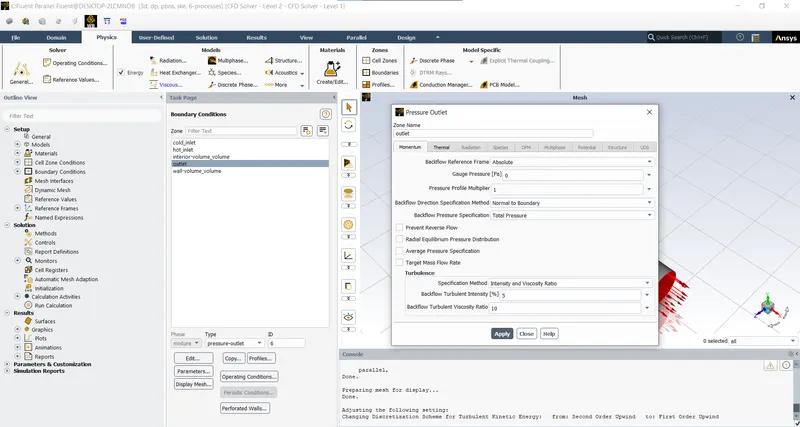
- Outlet as the Pressure outlet:
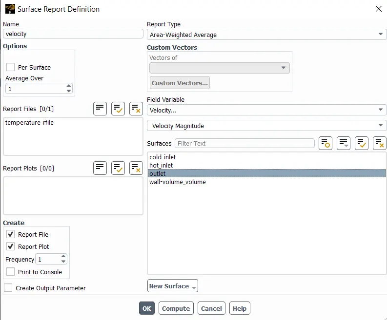
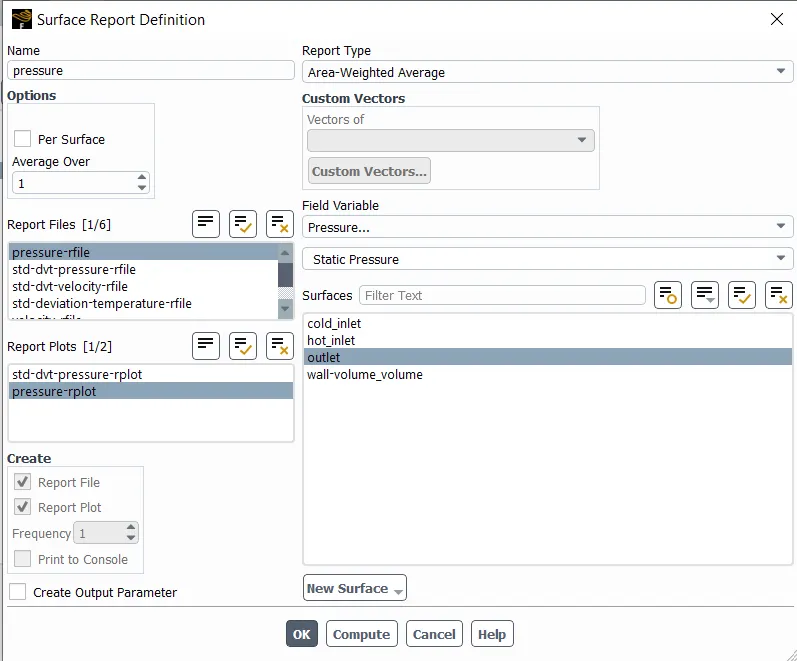
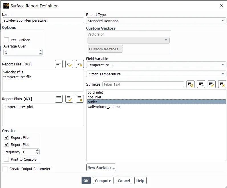
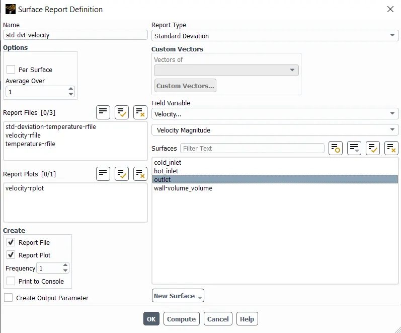
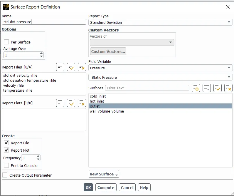
- Defining the Report Definitions (Solution > Definitions > New > Surface Report > Area wieghted average > Temperature/Velocity/Standard Deviation):
- To visualize the variations of the parameters the report plots are setup so as to check the convergence when there is no/negligible variation in output of the parameters.
- To visualize the report on the simulatio click rplot(To plot) and rfile(to keep the file).
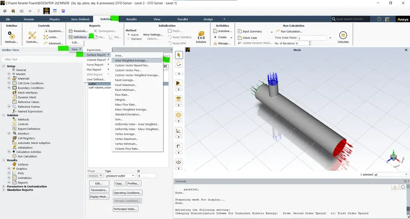
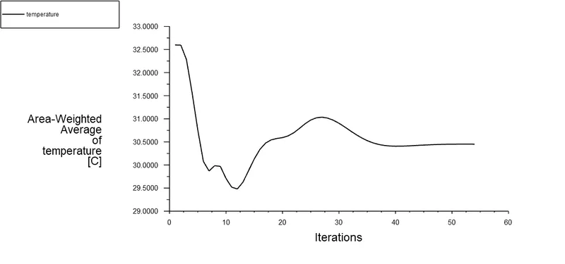
- For Temperture:
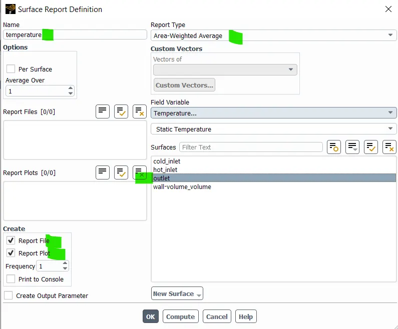
- Rename the report to the desired and select the area weighted average for the Temperature at the Outlet of the Tee.
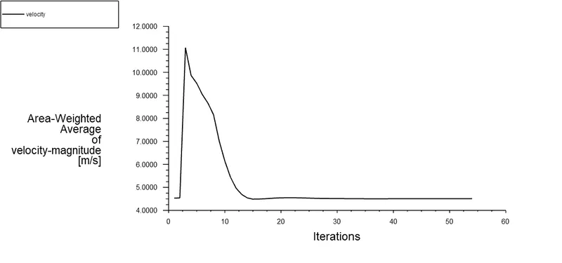
- For Velocity:
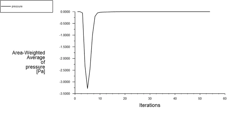
- For Pressure:
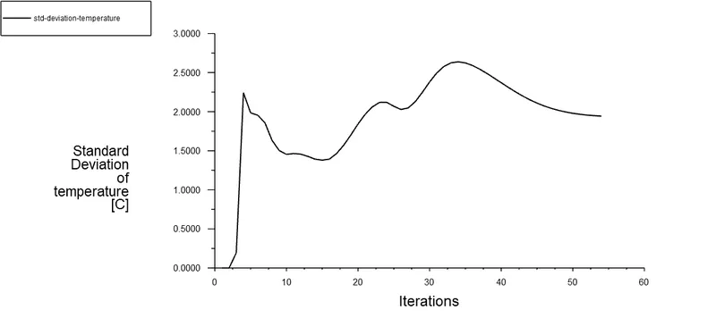
- Because we are concerned with the calculation of the mixing effectiveness we need to have the standard deviation of the temperature
- For Standard Deviation of the Temperature:
- For Standard Deviation of the Velocity:
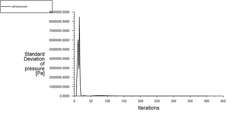
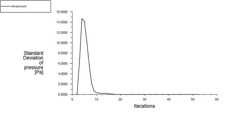
- For Standard deviation of the pressure:
- Using the double precision for the solver setup and parallel cores:
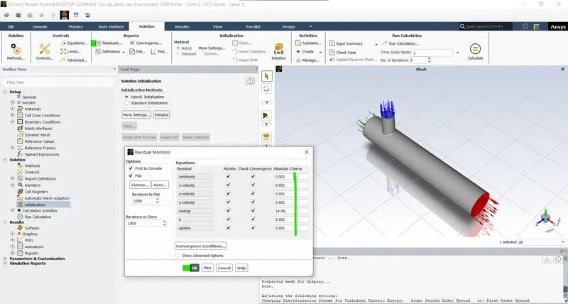
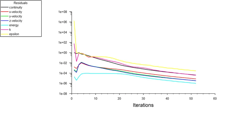
- Residuals:
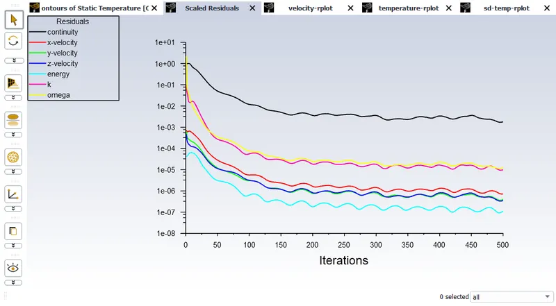
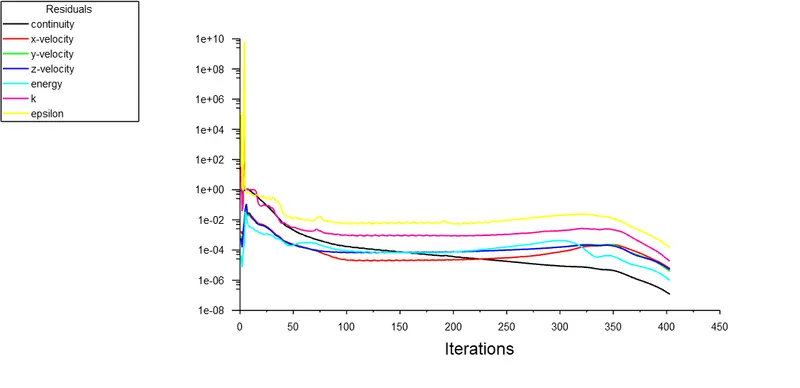
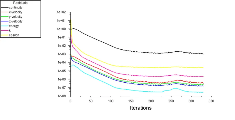
- These residuals show that what paramters are convered based on the predefined criteria of the output with respect to the iterations:
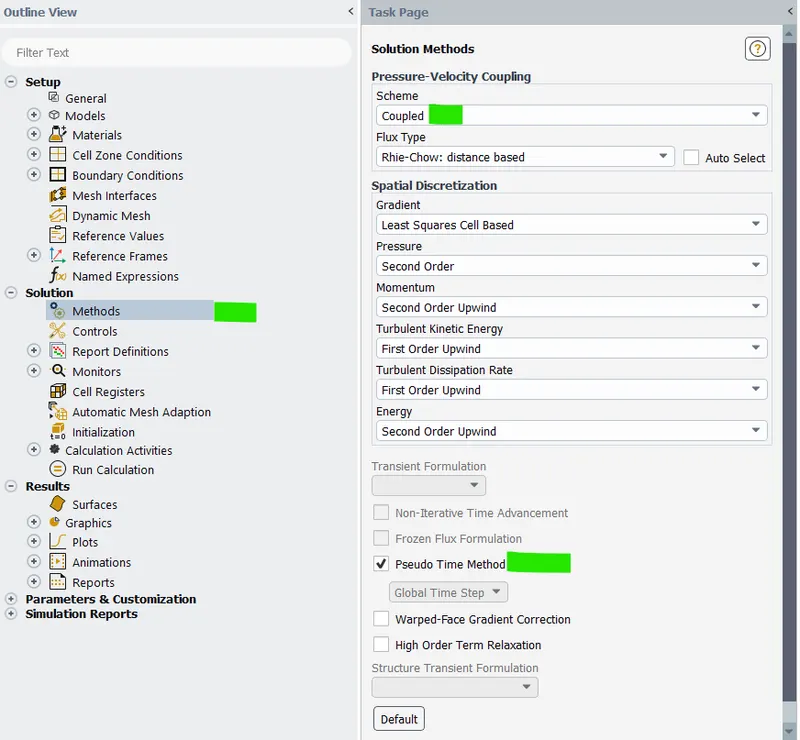
- In the Solution Method using the coupled scheme for the solver with pseudo time method:
- Now initializing the solver using the Hybrid Initialization:
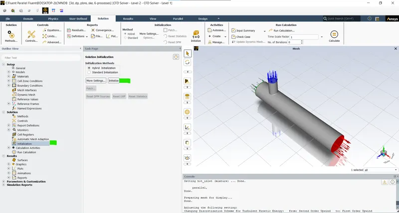
- The hybrid initialization uses potential solver to get the approximate values of velocity and pressure data.
- Initialization represents the asigning of the initial values to which the entire simulation is solved, here the solution is gused for the Euler Equation.
- The hybrid initialization solves the simulation with only the given data at the ideal conditions.
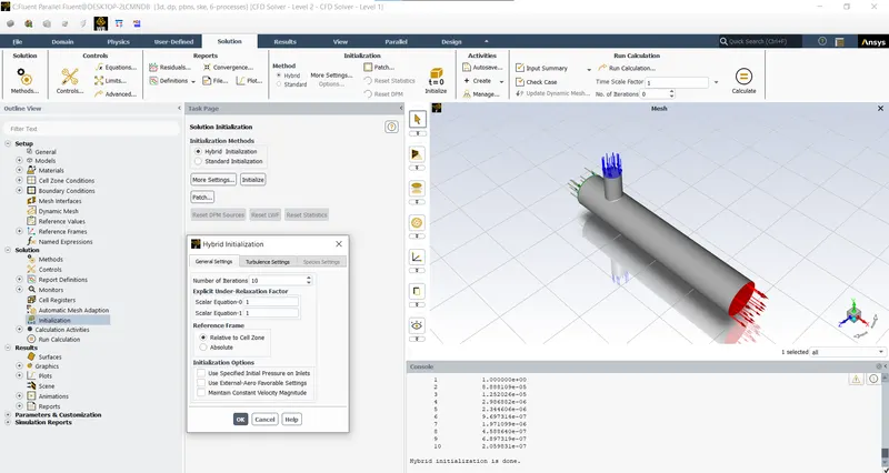
- The hybrid initialization is completed.
- Now solving till the solution is converged:
- Setting the iterations to 500 so make sure the solution converges with in it:
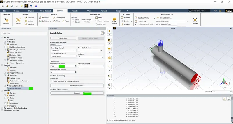
- The solution is converged after 54 iterations:

- Reports (Reports > Surface Integrals > Area weighted average > Select the Parameter > select the surface > Ok):
- To obtain the results about the parameters like temperature pressure and velocity at the outlet the surface plots are used with the area weighted average (to show the average parameter of the surface):
- For temperature:
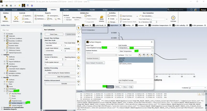
- Now obtain all the necessary parameters as stated above.
- To retrieve the data of the parameters after simulation use Reports > Surface Integral > Area weighted average > Parameters > At surrface > compute:
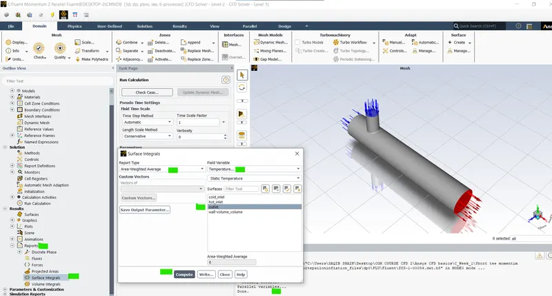
- Area weighted average gives the average value of the set parameter at given surface.
- Post-Processing:
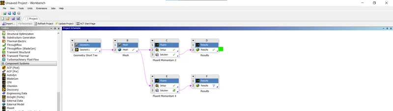
- Open the results in the component system:
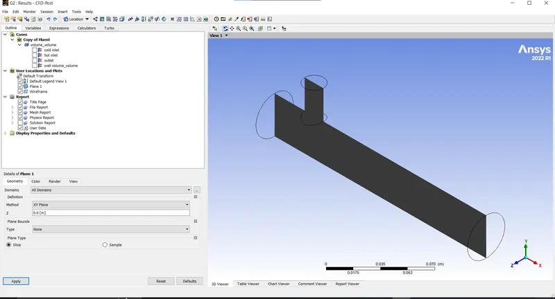
- Now to visualize the properties we insert a plane in the middle i.e. centre of the planes in xy plane as the gemetry is symmetrical in this plane (Location > Plane > xy plane > 00 > ok):
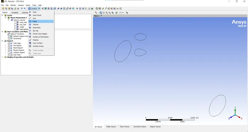
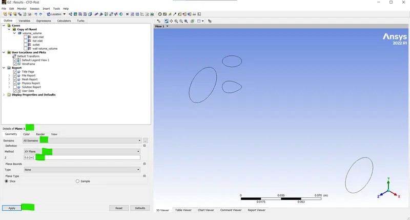
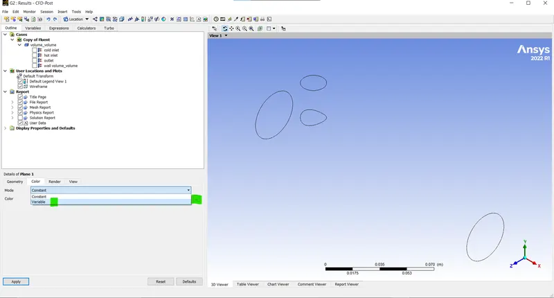
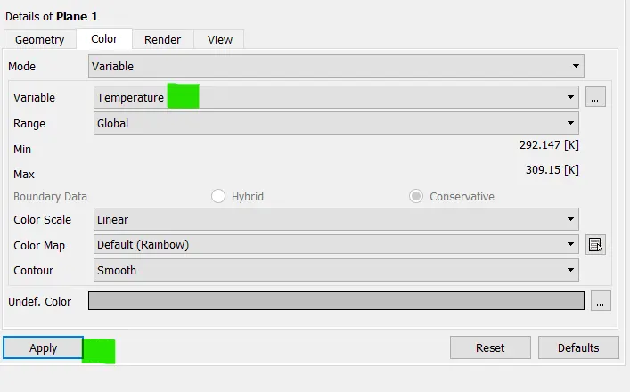
- Now select the variable option in the mode tab and choose the parameter to be represented:
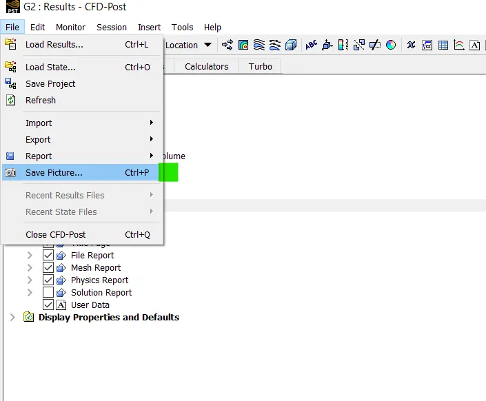
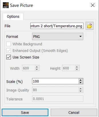
- To save the contour plots:
- File > Save Picture > Name > Ok.
- For line plots:
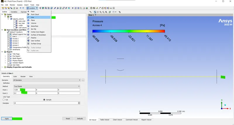
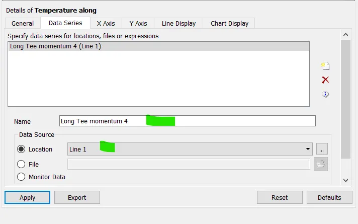
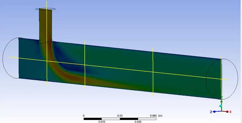
- Create a line with sample option and the approximate co-ordinates (Location > Line > Enter co-ordinates > Chart > Define x-axis > Define y-axis > Plot):
- To create the plots:
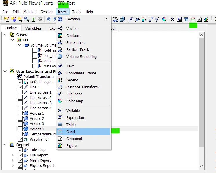
- Select the chart option from the tool bar (Insert > Chart):
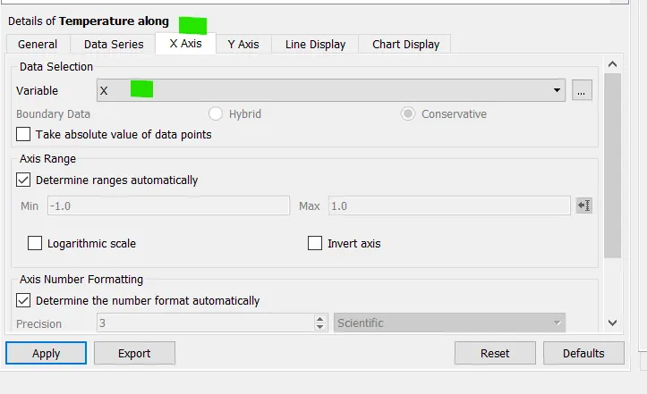
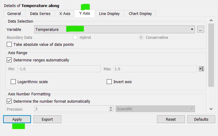
- Now define the x-axis and y-axis for the respective plots:
- Give the series name and the tilte for the respective chart:
- Select the location on to which the chart is needed:
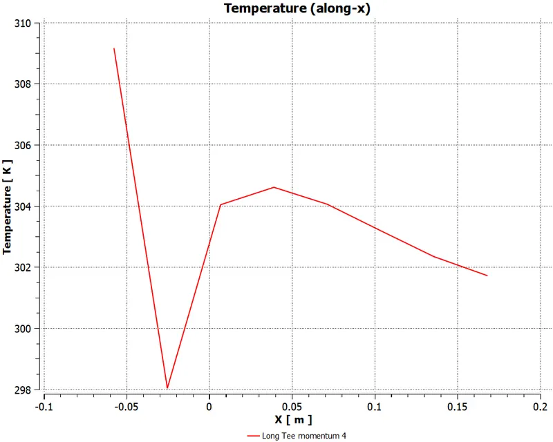
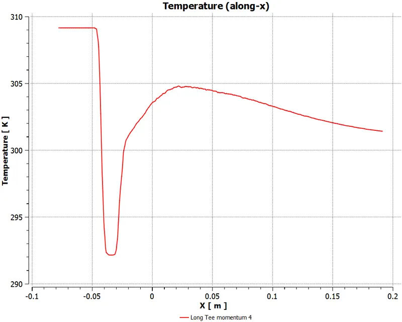
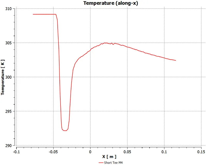
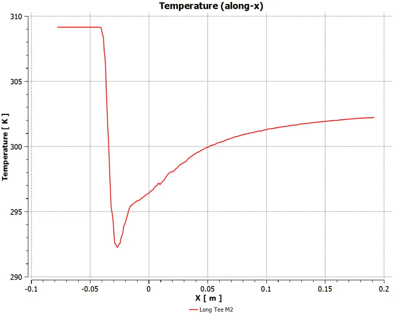
- Here for along the length of the Tee the x- axis is length of the Tee in the x-direction:
- And the y-axis are the parameters fo example temperature:
- Save the chart (File > Save Picture > PNG > OK):
- Increasing the sample size to max - 1000:
- Select the chart option from the tool bar (Insert > Chart):
- Create a line with sample option and the approximate co-ordinates (Location > Line > Enter co-ordinates > Chart > Define x-axis > Define y-axis > Plot):
- Open the results in the component system:
- For Short tee with momentum 2:
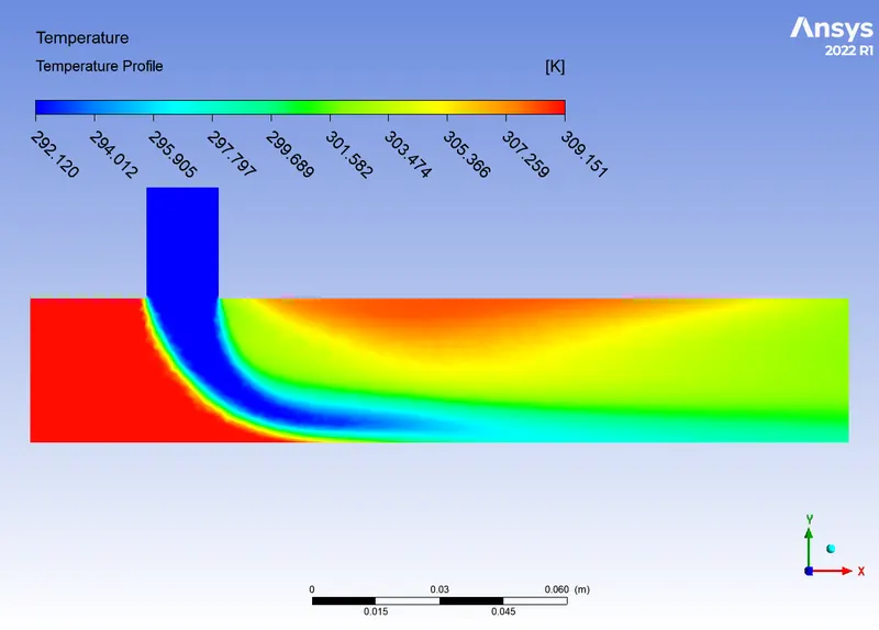
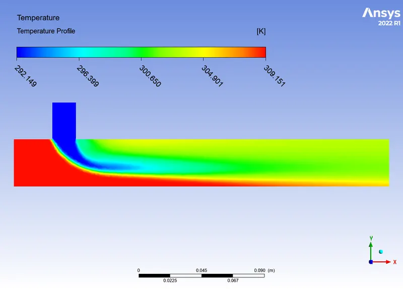
- Temperature profile:
- Velocity Profile:
- Temperature profile:
- Selection of the model for the solver:
- k-omega SST model:
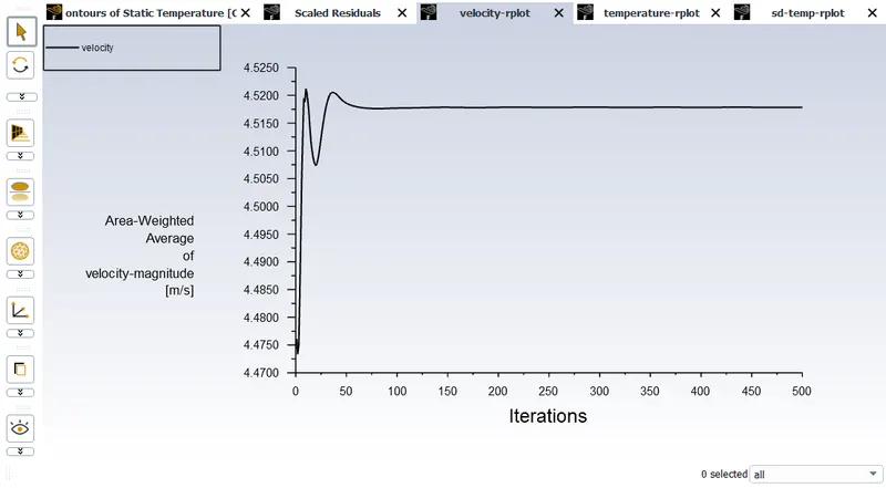
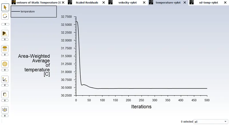
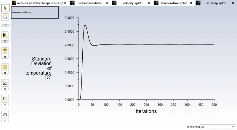
- Convergence/Residuals:
- Temperature contours:
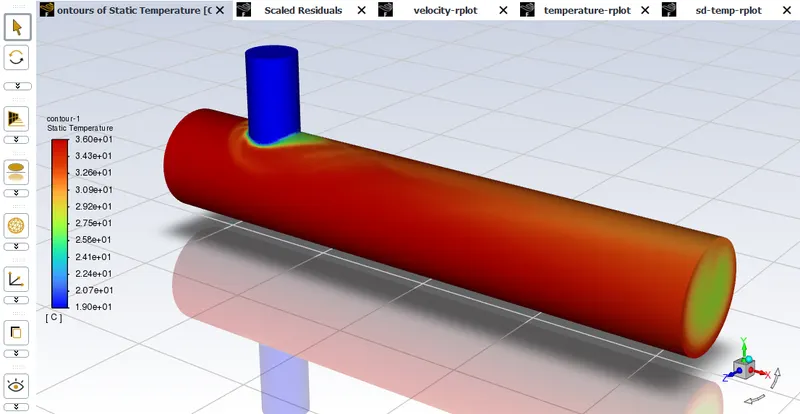
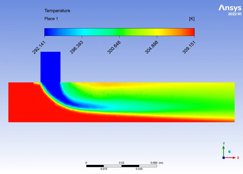
- Temperature profile:
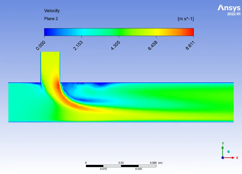
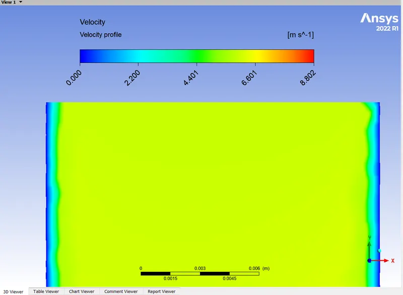
- Velocity profile:
- k-epsilon mode:
- Residuals:
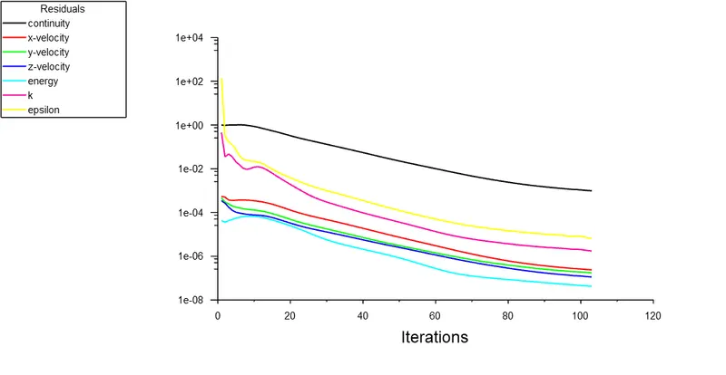
- Standard deviation of temperature and pressure:
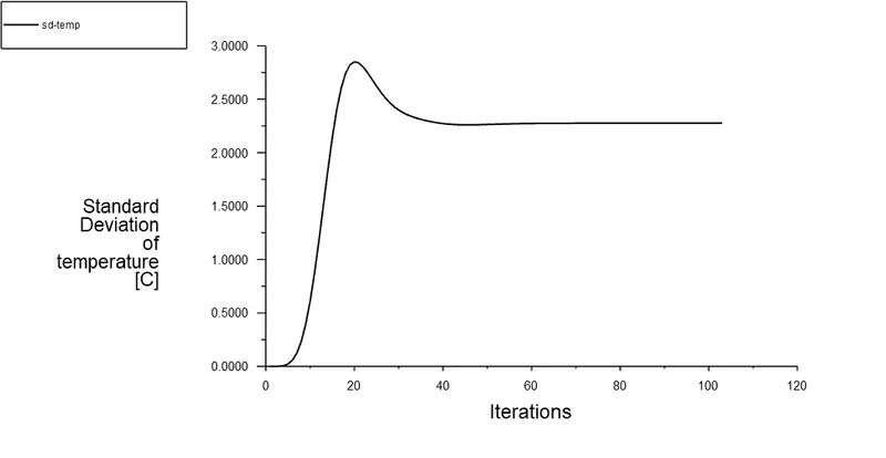
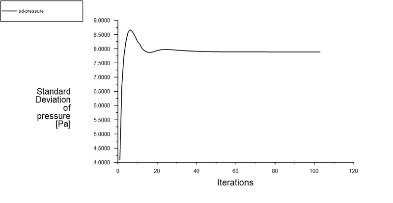
- Temperature and velocity:
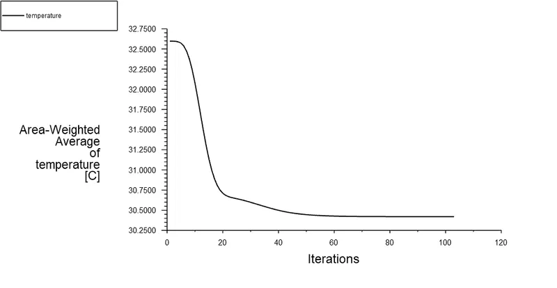
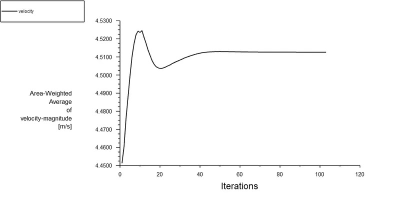
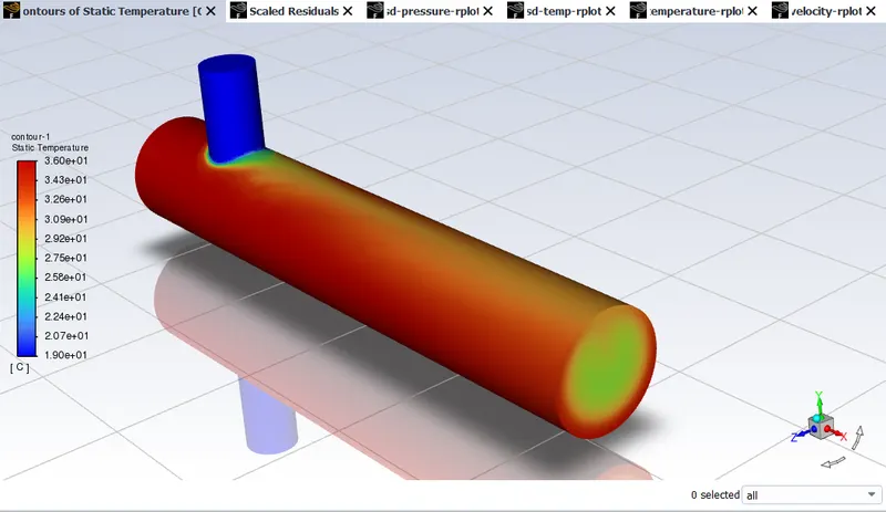

- ResultsOutputs converged at 103 iteration.
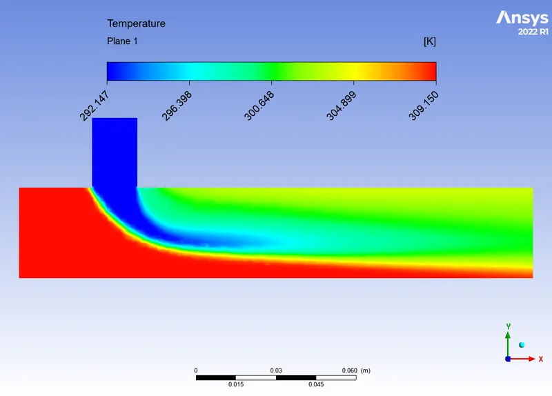
- Temperature profile:
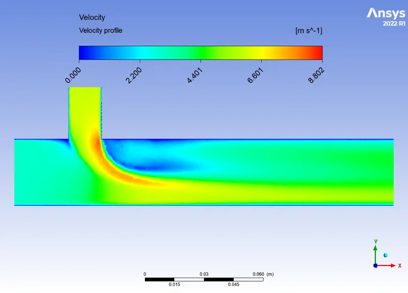
- Velocity profile:
- k-epsilon model (with Inflation layers):
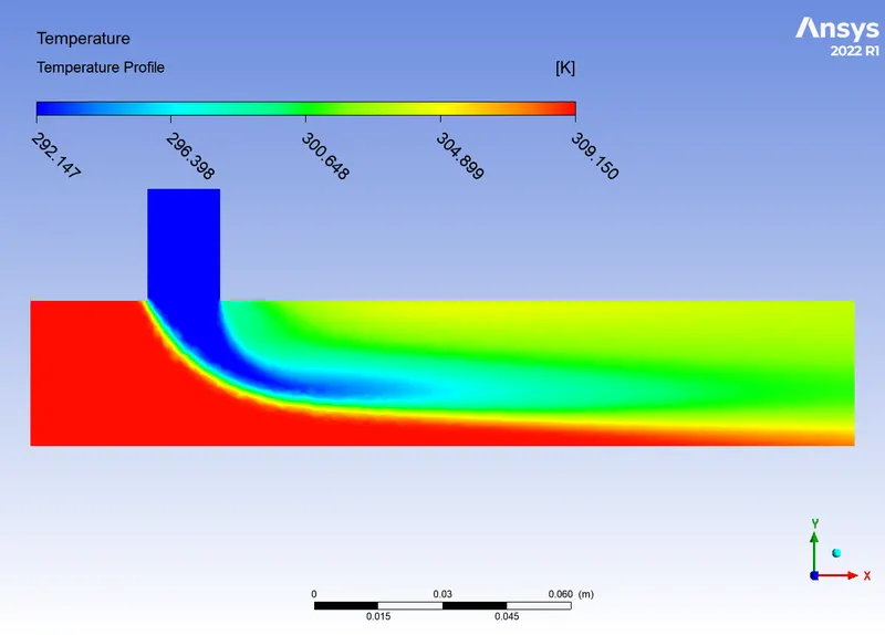
- Temperature Profile:
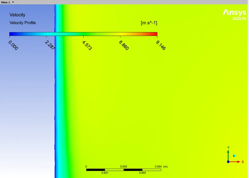
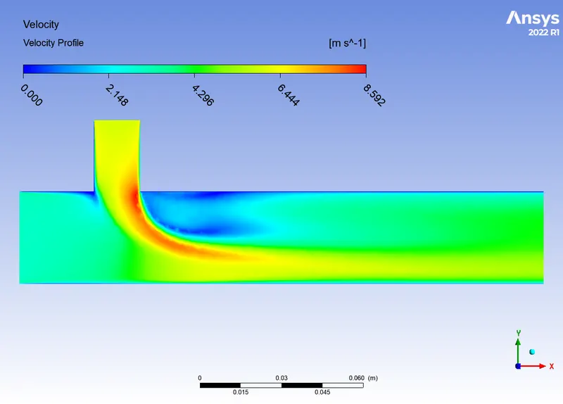
- Velocity:
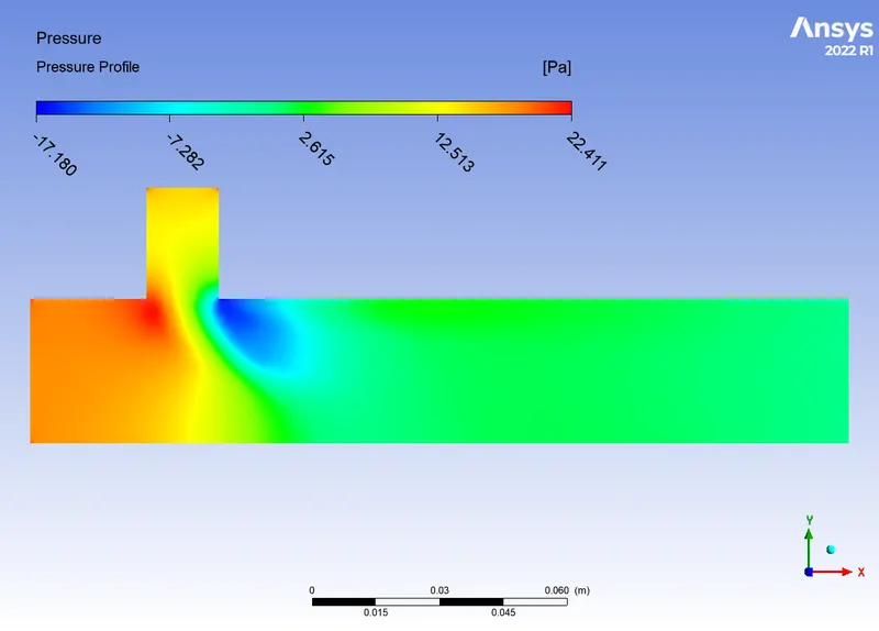
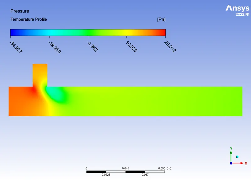
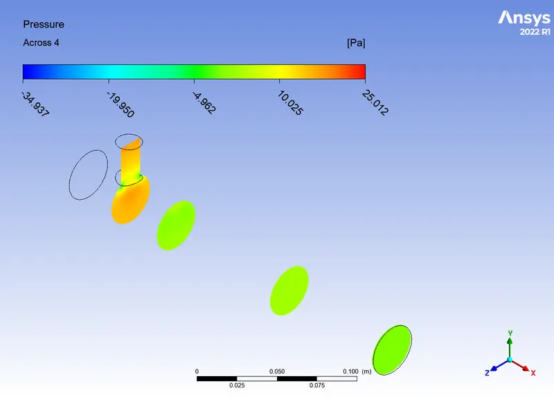
- Pressure Profile:
- The k-epsilon model is used to study the free shear layers and the wake regions in the flow but dosn't have much to provide in the near wall boundary regions.
- The standard k-omega model is used to study the near wall conditions in the fluid dynamics as it provides more accurate results than the k-epsilon model.
- There is an improved HYBRID version of the k-omega model known as k-omega SST which uses k-epsilon and Wilcox k-omega model and deploys over the requisite domains of the fluid flow i.e. for the free stream region k-epsilon and for the near wall regions SST k-omega.
- k-omega SST model:
-
- As seen above the k-omega SST model didn't converge even for 500 iterations but k-epsilon model converges more quickly compared to k-omega SST.
- Here in this study we are only concerned over mixing effectiveness of the flow not the near wall regions so the k-epsilon model can be used as it provides the reqired data and converges more easily than the SST k-omega model.
- Now open the mixing tee in the meshing environment(Mesh > Edit > ok):
Results:
- For Short Tee (Momentum Ratio = 2):
- Residuals:
- Temperature(c):
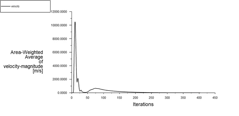
- Velocity(m/s):
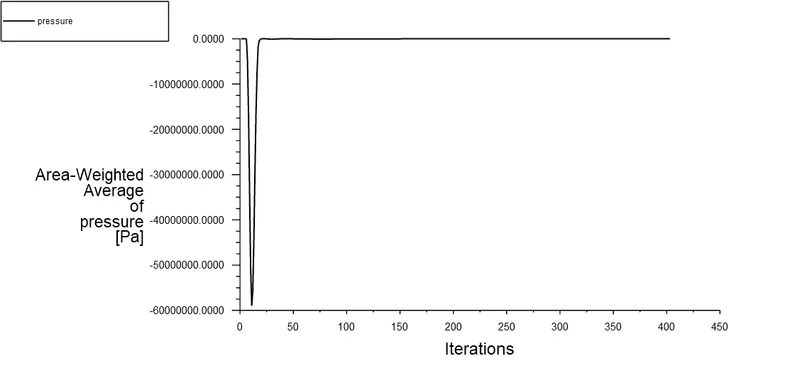
- Pressure(Pa):
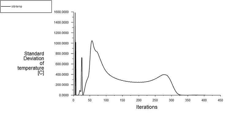
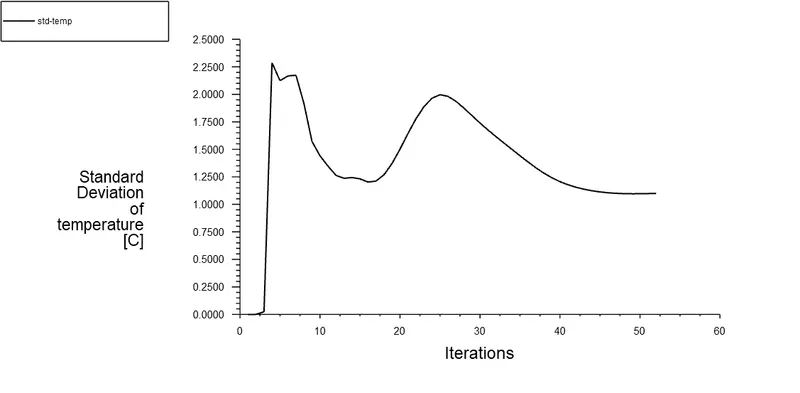
- Standard Deviation Temperature:
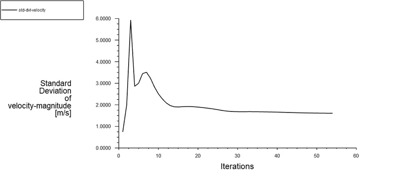
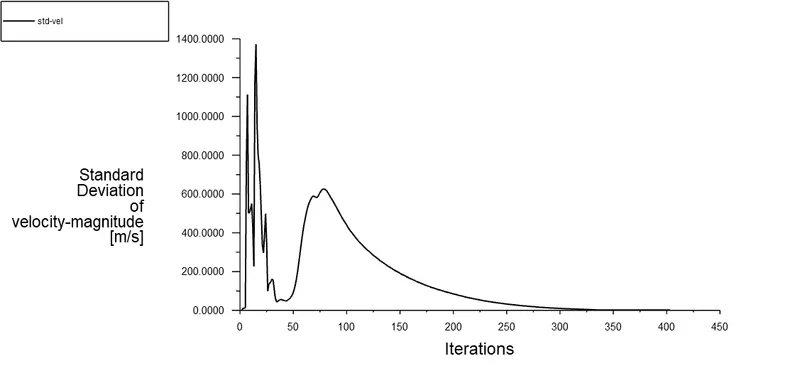
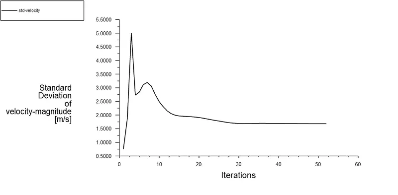
- Standard Deviation Velocity:
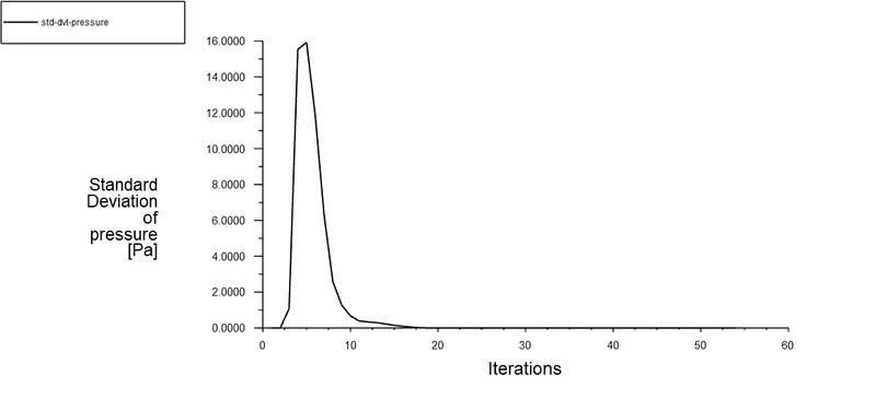
- Standard Deviation Pressure:
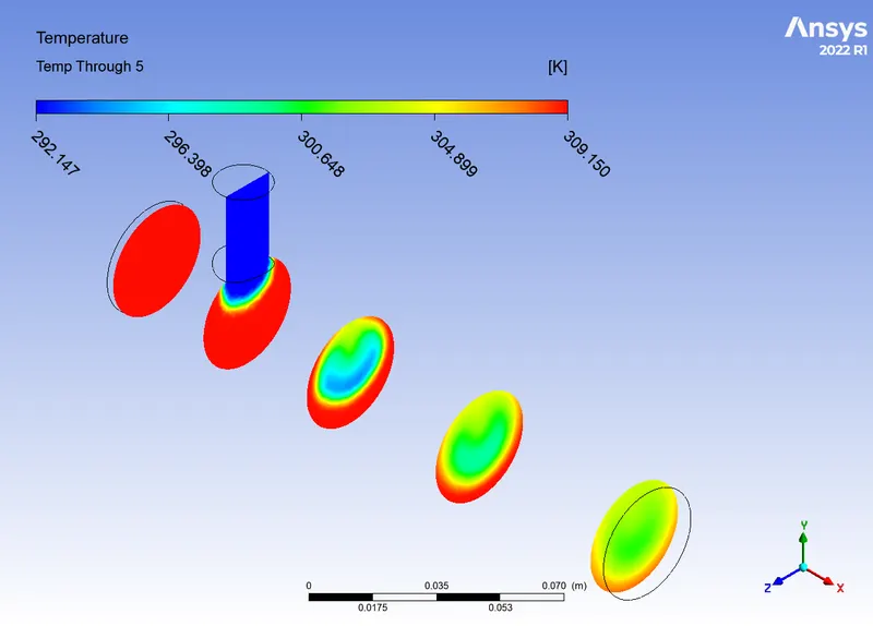
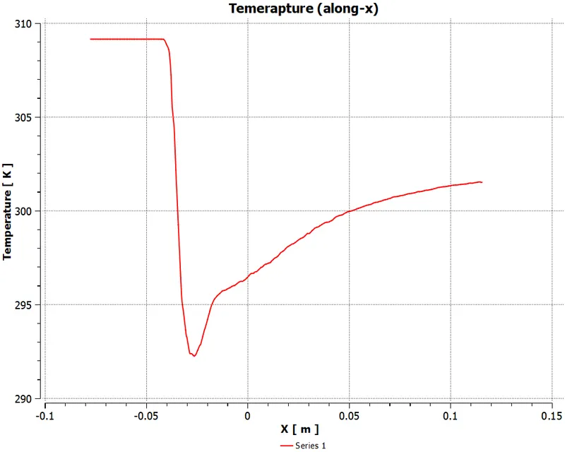
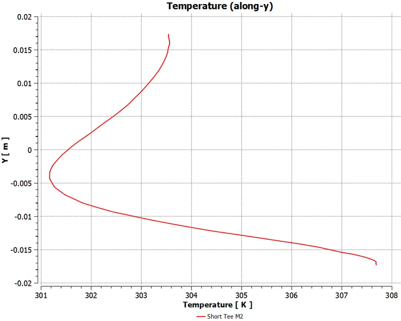
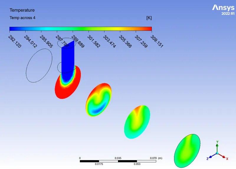
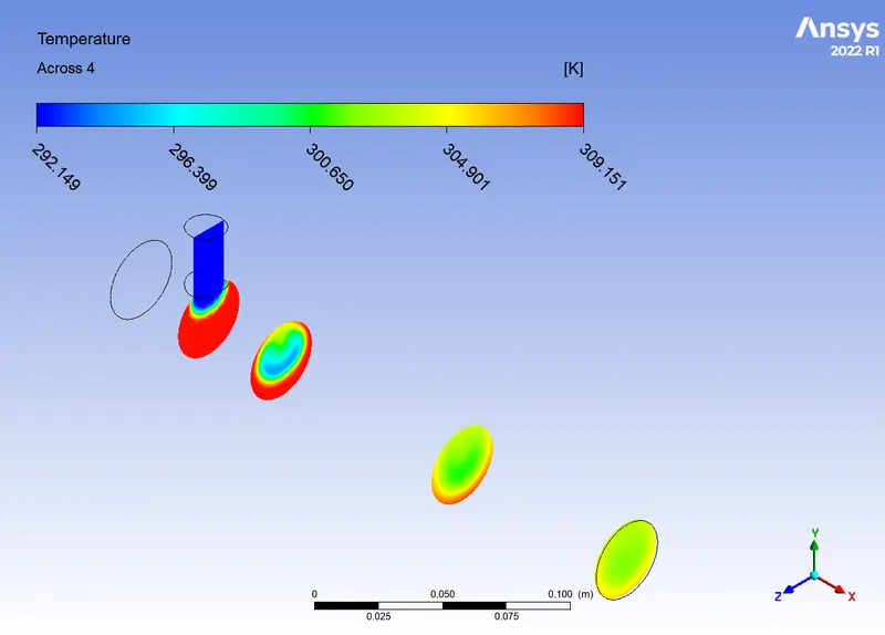
- Temperature Profile and Line Plots:
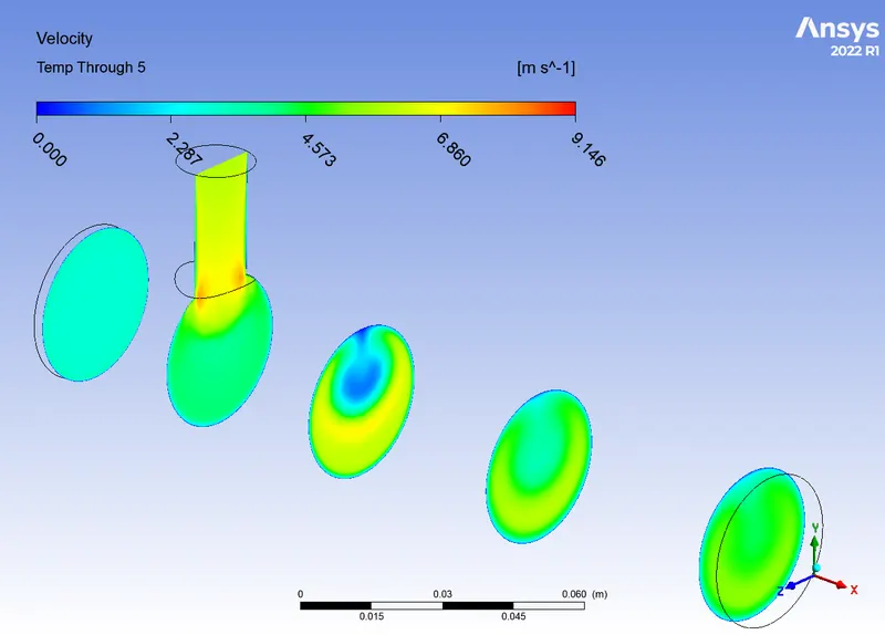
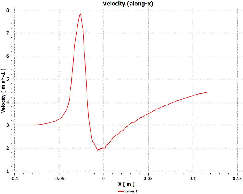
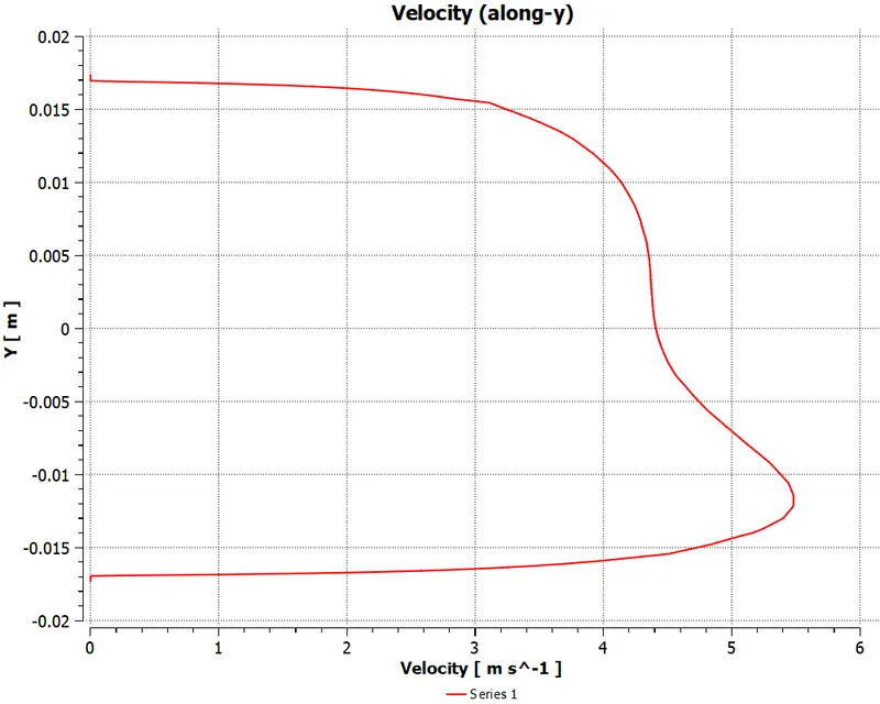
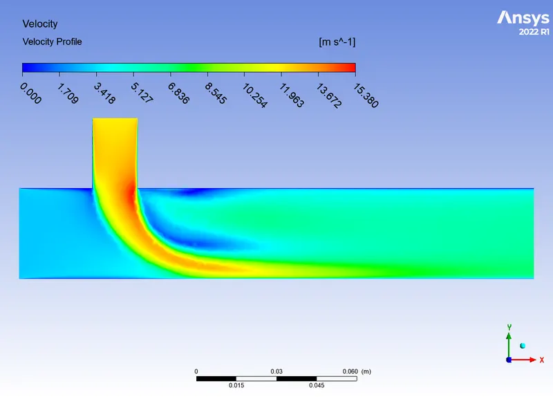
- Velocity Profile:
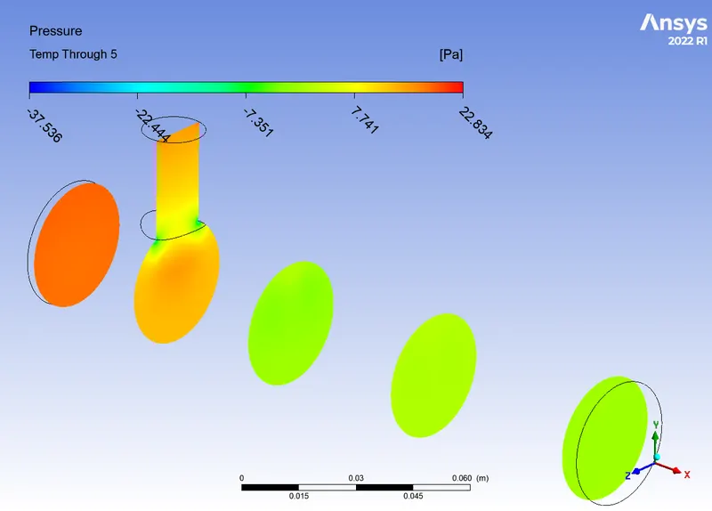
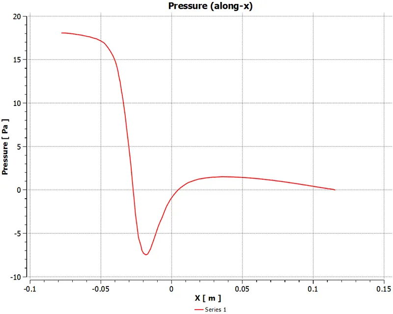
- Pressure Profile:
- Residuals:
- For short tee (Momentum Ratio = 4):
- Residuals:
- Temperature Convergence:
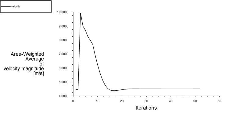
- Velocity convergence:
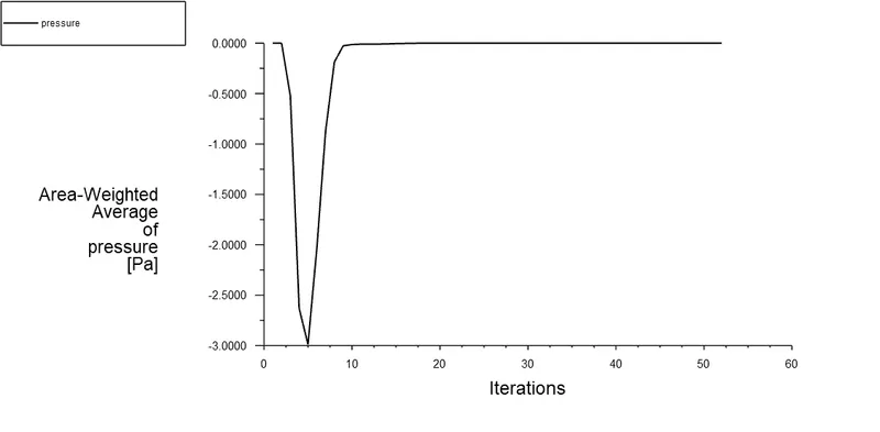
- Pressure convergence:
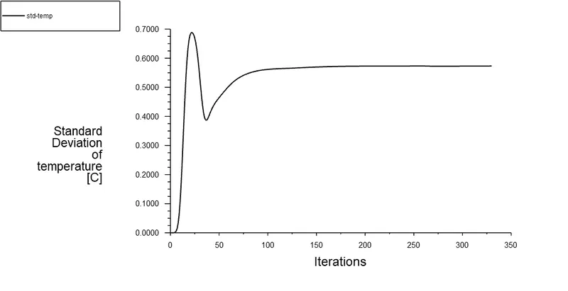
- Standard deviation of Temperature:
- Standard deviation of Velocity:
- Standard deviation of pressure:
- Temperature Profile and plots:
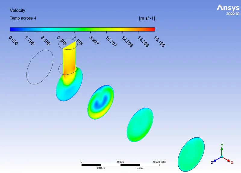
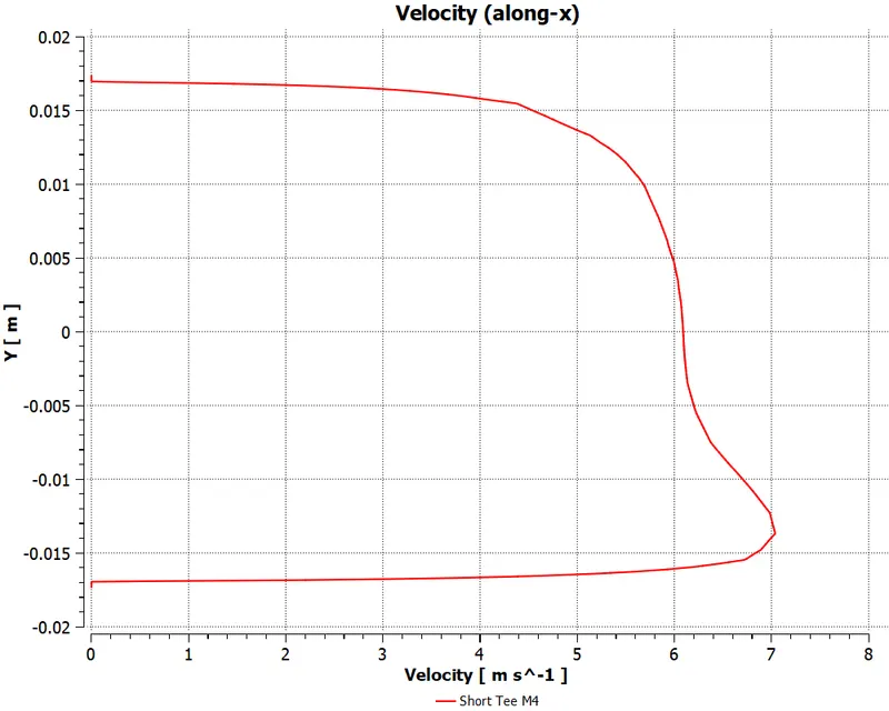
- Velocity Profile:
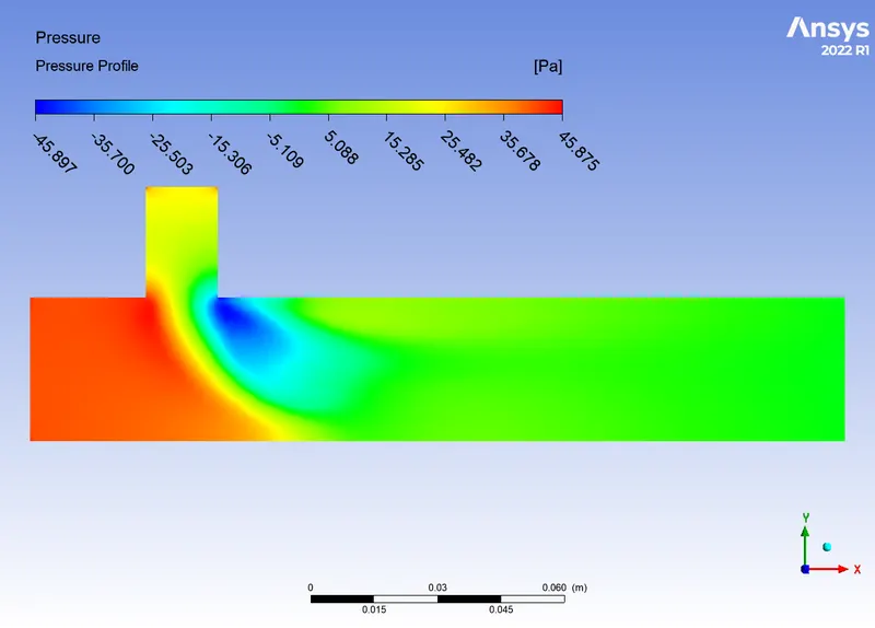
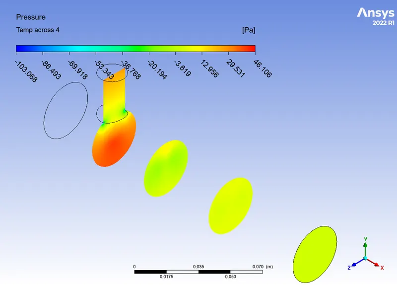
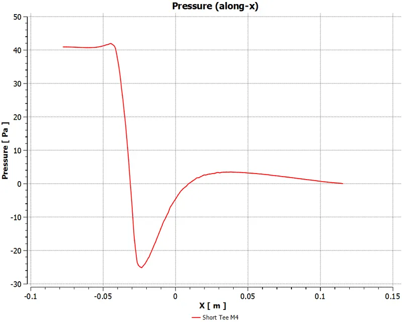
- Pressure Profile:
- Iterations to converge:
- Residuals:
- Long Tee (Momentum Ratio = 2):
- Mesh:
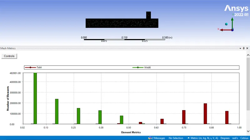
- Element quality(Mesh metrics):
- After removing the inflation layers:
- Residuals:
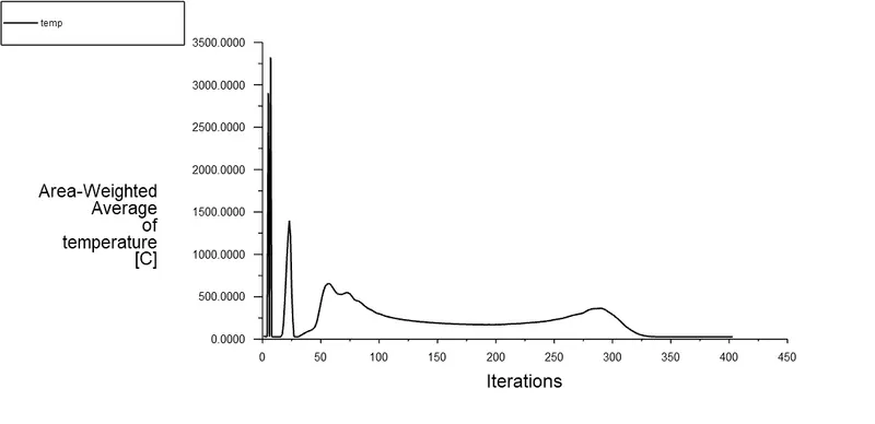
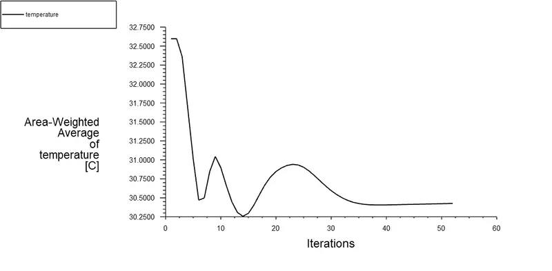
- Temperature convergence:
- Velocity convergence:
- Pressure convergence:
- Standard deviation of Temperature (at outlet):
- Standard deviation of Velocity (at outlet):
- Standard deviation of Pressure (at outlet):
- Temperature Profile and plots:
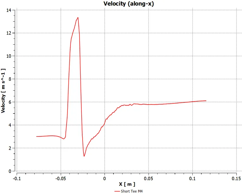
- Velocity Profile and plots:
- Pressure Profile:
- Mesh:
- Long Tee (Mometum - 4):
- Mesh(Elements Quality):
- As most of the elements are in the region of 0.8 we have acceptable mesh(0.4-0.8 acceptable).
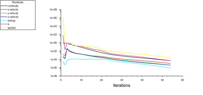
- Residuals/convergence:
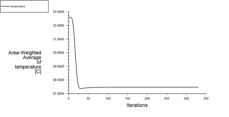
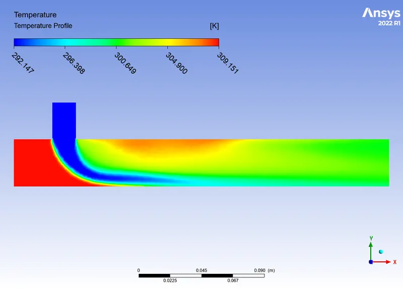
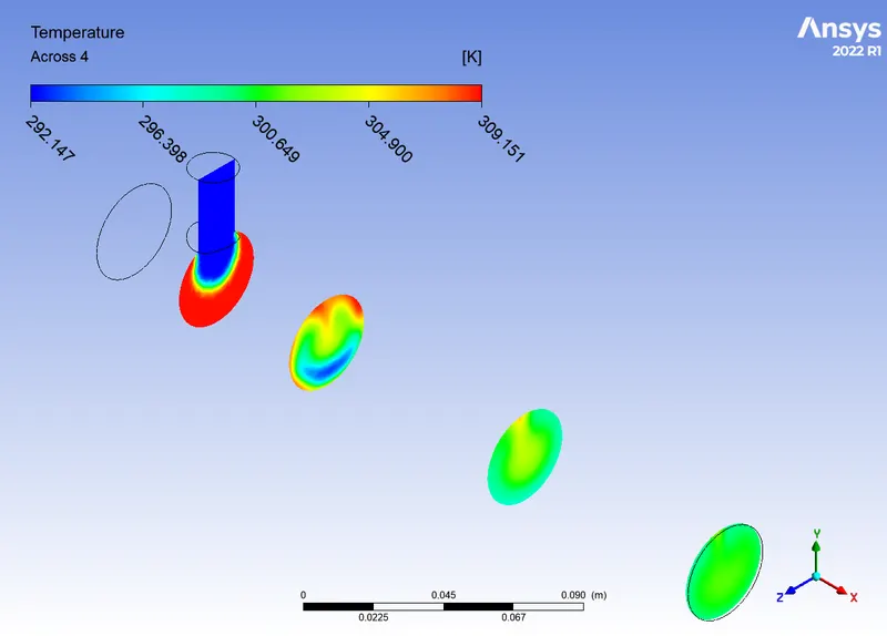
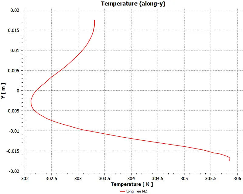
- Temperature Convergence and profiles:
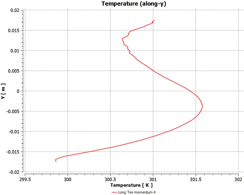
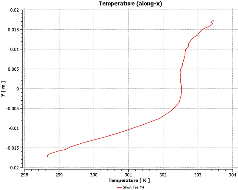
- At outlet (Y-axis = y distance, X-axis = Temperature):
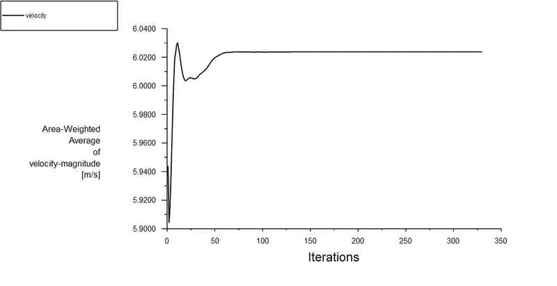
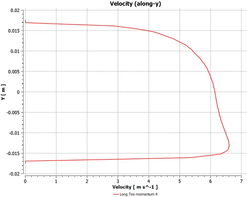
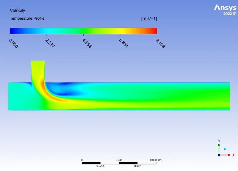
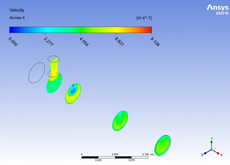
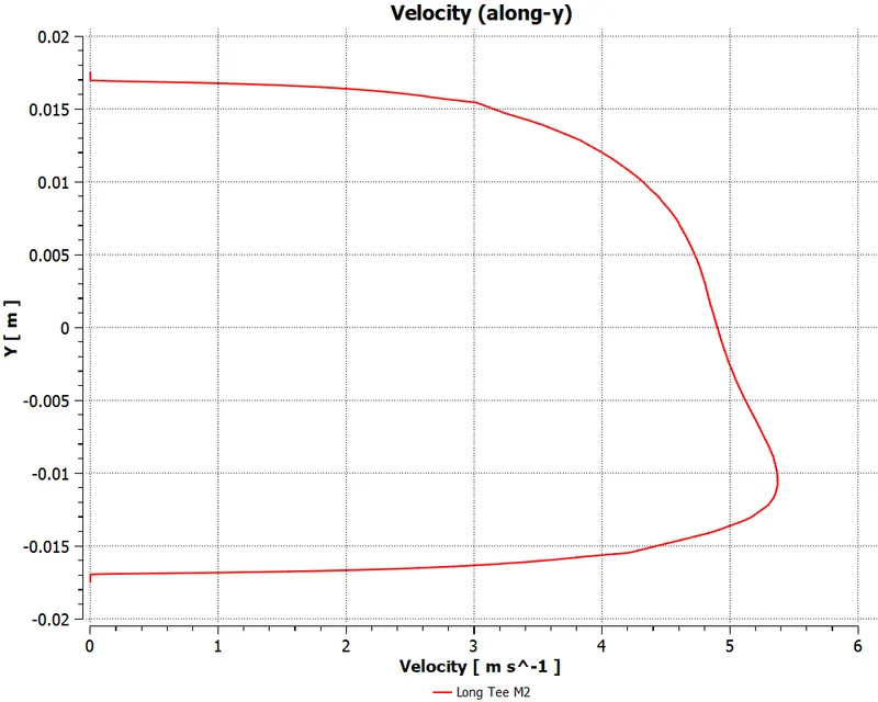
- Velocity Convergence and profiles:
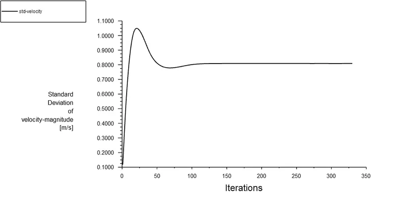
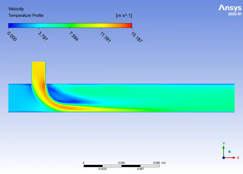
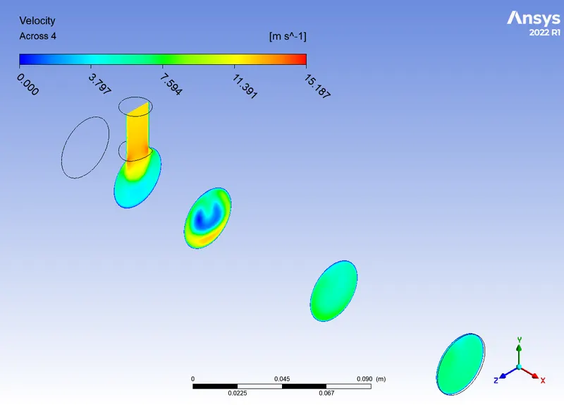
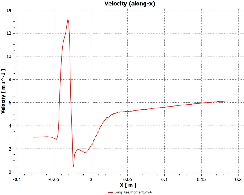
- At outlet (Y-axis = y distance, X-axis = velocity):
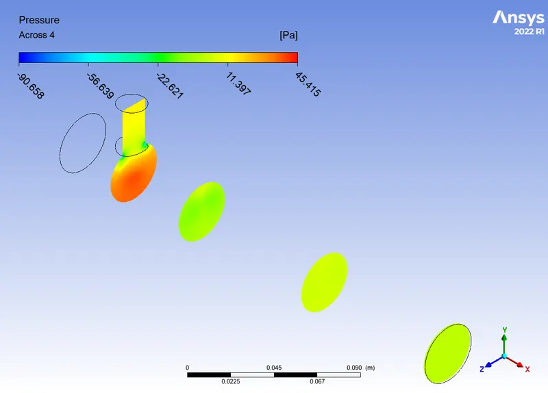
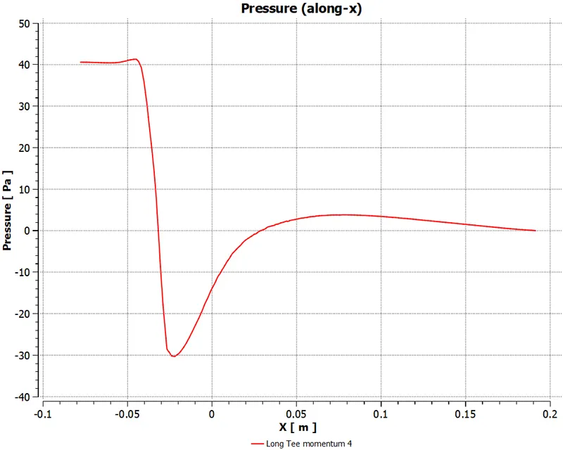
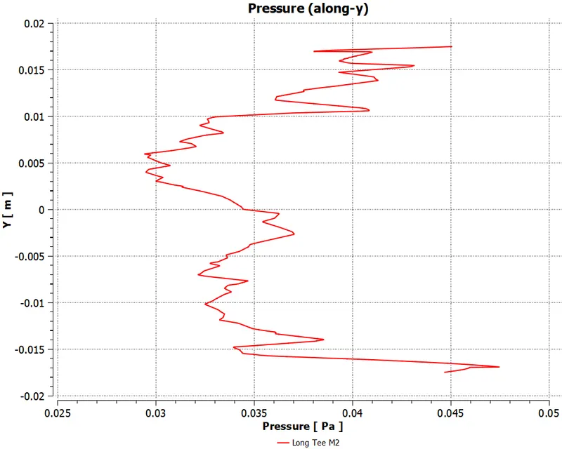
- Pressure Convergence, profiles and plots:
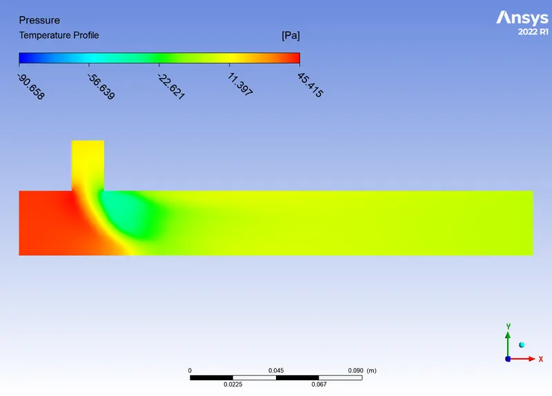
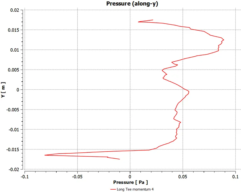
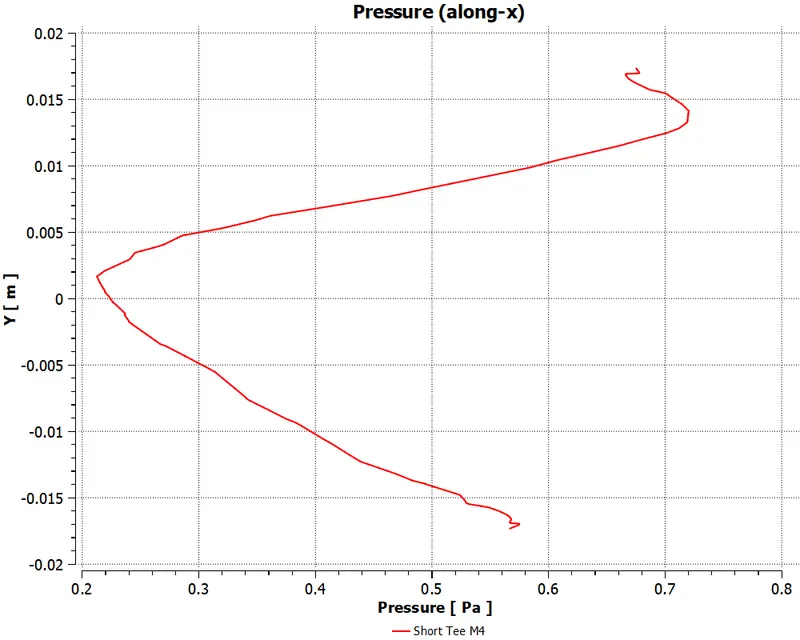
- At output(Y-axis Distance in Y, X-axis = Pressure):
- Mesh(Elements Quality):
- Results table:
-
Sl.no Case type Momentum Cell Count Iter to conv Outlet (Area weighted average) Inlet (Area weighted average) Error (temp) Temperature (act) (c) Temperature (Thro) (c) Velocity (m/s) Pressure Hot (Pa) Pressure Cold (Pa) 1 Short Tee 2 1165603 54 30.451136 30.3290279 4.5091 18.456403 16.05448 0.40099688 2 4 1165603 403 27.483789 27.4951573 6.0381 41.297582 28.262116 0.0413637 3 Long Tee 2 1576412 52 30.425633 30.3290279 4.5043 20.630497 18.233004 0.31751222 4 4 1576412 (765896) 330 27.470758 27.4951573 6.0237 40.788054 15.447276 0.08881918
-
- Note: Inflation layers were deleted as they were causing unwanted warnings/errors, it doesn't concern as the results were steady state and converged without any errors(Back Flow and Failed Computation), simulations were rerun to reference the previous output results.


Geometry (Meshed):
- With Inflation:
- Without Inflation:
Conclusions:
- The geometry is meshed and the mesh independeny test is conducted and 1mm element length is found to be more suitable for the study.
- The k-epsilon model is selected for this case of simulation as we are not more concerned with the near wall conditions but only the mixing effectiveness.
- The simulation is completed successfully, the procedure and results are explained in detail above.
- The Mixing effectiness greatly affected by the momentum ratio i.e. Relative velocities of the inlet fluids, as more velocity of the fluids tends to create more turbulence and hence provide better mixing.
- The Length doesn't seem to have an major affect on the mixing as observed from the simulation study.
- Even though there is more diffusion in the longer pipes (Increased diffusion cone) it doesnt have any major and significant effect on the mixing of the fluids(Only minor - second decimal change).
- For the optimized better results it advised to use the Short Tee with momentum ratio 4.
- If still the enhanced results are needed used the longer Tee for the process.
- The outputs and the conditions are tabulated below:
References:
- Two-equation eddy-viscosity turbulence models for engineering applications F. R. Menter AIAA Journal 1994 32:8, 1598-1605
- Menter, F.L.O.R.I.A.N.R., 1993, July. Zonal two equation kw turbulence models for aerodynamic flows. In 23rd fluid dynamics, plasmadynamics, and lasers conference (p. 2906).
- Torabi Asr, Mahdi. (2015).