Week 4 - CHT Analysis on Exhaust port
Aim: Perform the conjugate heat transfer analysis on the exhaust port with the appropriate parameters and verify it with the therotical results.
Objective:
- Clean the geometry.
- Mesh the geometry.
- Perform the grid independent study.
- Run the simulation.
- Verify the numerical results.
Theory:
- Conjugate heat transfer:
- Conjugate heat transfer refer to the heat transfer were both conduction and convection occurs simultaneously.
- Conduction being dominant in the solid and no slip region and convection being dominant in the fluid region.
- In other words it can be said that conjugate heat transfer analysis refers to the simulation of heat energy transfer between the solid and fluid at the interface.
- Modes of heat transfer:
- There are three modes of heat transfer:
- Conduction: Here the heat energy is transfered due to the lattice vibration or due to dislocation of the electrons but there is no net disslocation(no mass movement).
- Here the heat energy transfer is governed by the Fouriers law which state that the heat transfer through the medium due to conduction is directly proportional to the normal area and the negative temperature gradient and inversly proportional to the distance through the medium.
- It is given by:
- `Q = -kA(dt/dx)`
- Units = watts.
- Negative sign indicates the negative temperature gradient.
- k is the proportionality constant i.e. Thermal conductivity (W/m.k)
- A is the area normal to the heat transfer direction.
- t is the temperature in k or celcius.
- 'x' is the distance.
- Convection: In convection the heat energy is transfered by the motion of the particles od the medium i.e. motion of the particles of the medium results in the transfer of heat energy, there are two types of convection:
- Natural/Free convection: Here the motion of the particles of the medium is due to the density difference caused due to the temperature gradient.
- Forced convection: Here the motion of the particles of the medium in addition to the motion due to density difference is produced by external devices such as pump, fans etc.
- The convection heat transfer is governed by the Newtons law of cooling which states that heat transfer through the fluid or between solid and the fluid surface is directly proportional to the temperature difference between the solid and the fluid or the fluid and fluid.
- Radiation: This is the type of the heat transfer mechanism which used electromagnetic waves for the transfer and also not requires the medium of propagation in contrast to the other mode of propagation.
- When conduction and convection occurs simualtaneously in a same study we can call it as the conjugate heat transfer.
Content of the body:
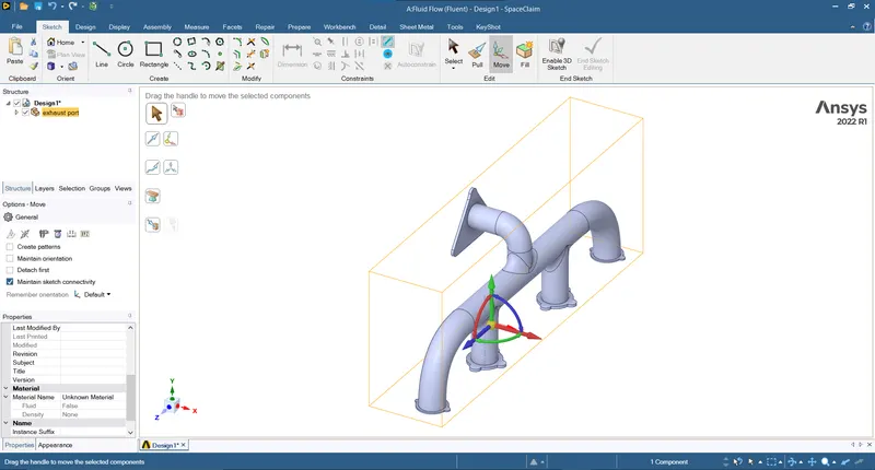
- Import the geometry into the spaceclaim (Drag and drop or used open in file):
- Check for any errors:
- Check for any extra edges (Repair > Extra Edges > Ok):
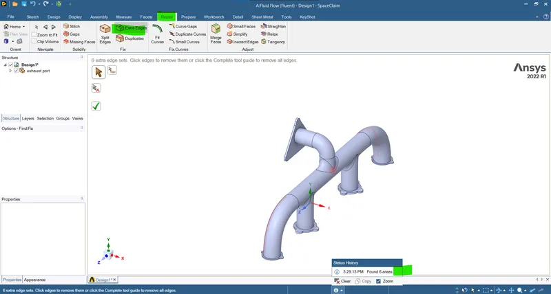
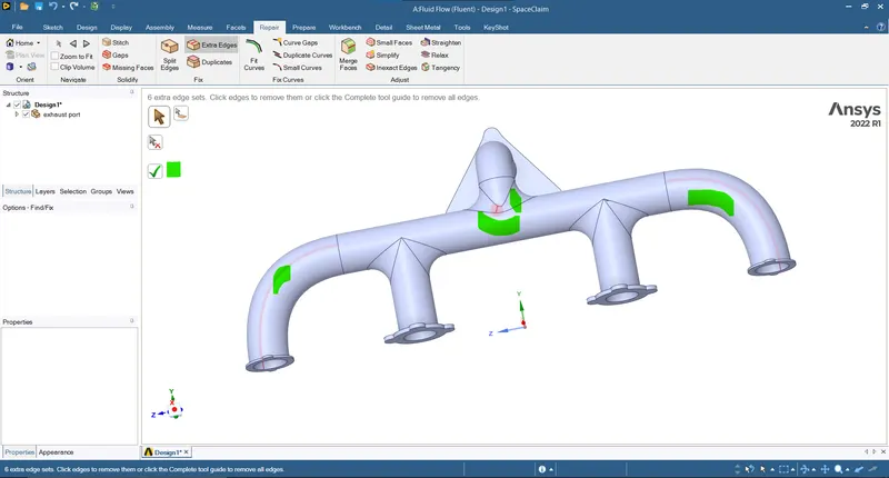
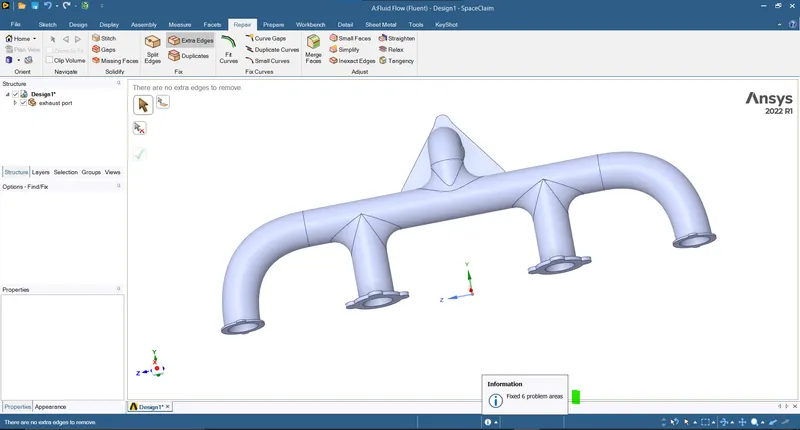
- Ass there are no other errors we can proceed to volume extract.
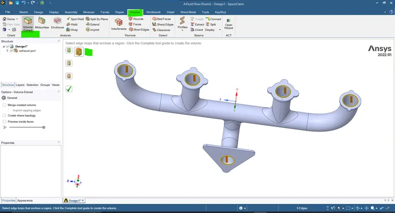
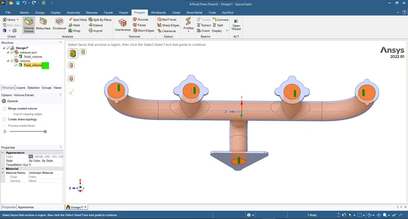
- Extracting the fluid volume. here the volume inside the manifold were the fluid exits is created as volume and the volumes are renamed (Prepare > Volume Extract > Select the edges to create the volume and Ok):
- Renaming the volumes:
- Solid volume:
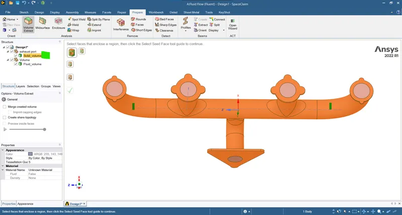
- Fluid volume:
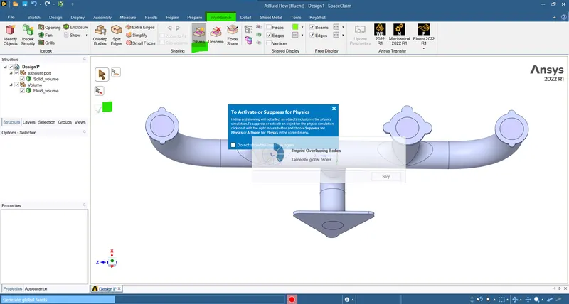
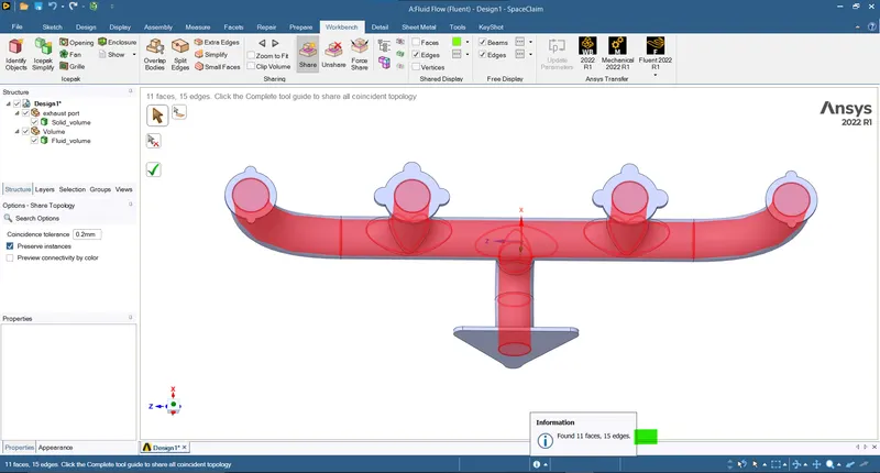
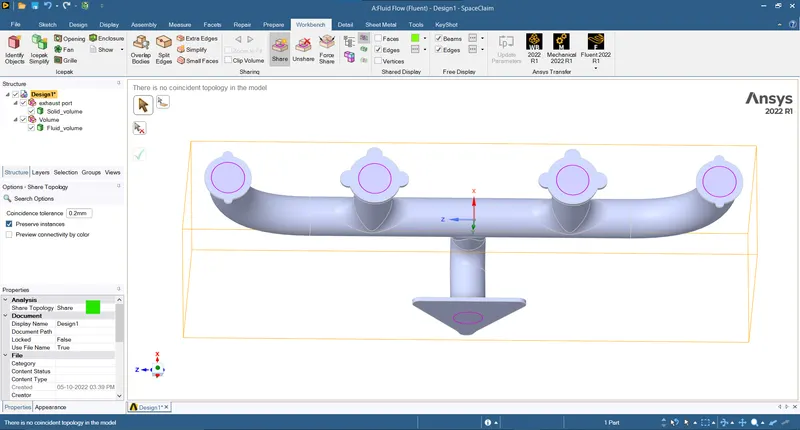
- Now sharing the topology to allow the data flow between the volumes (Workbench > Share > Ok):
- Now the work in spaceclaim is complete noww moving for meshing the geometry.
- Open the Mesh in the Fluent tab:
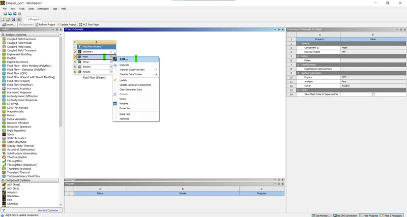
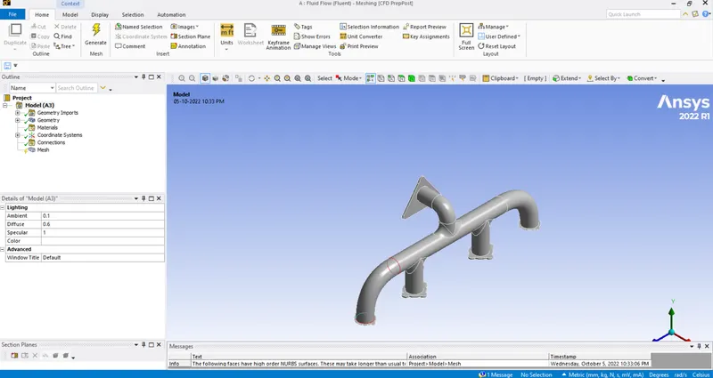
- Open the mesh (Right click > Edit > Ok):
- Now naming the components:
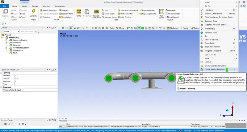
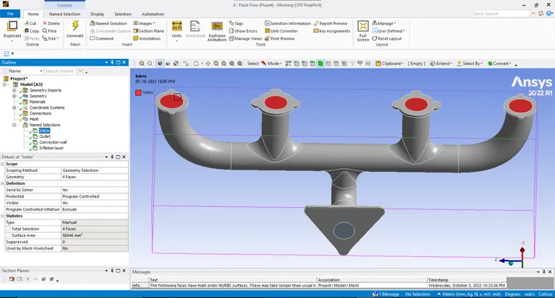
- Inlets (Select the surface and create named selections):
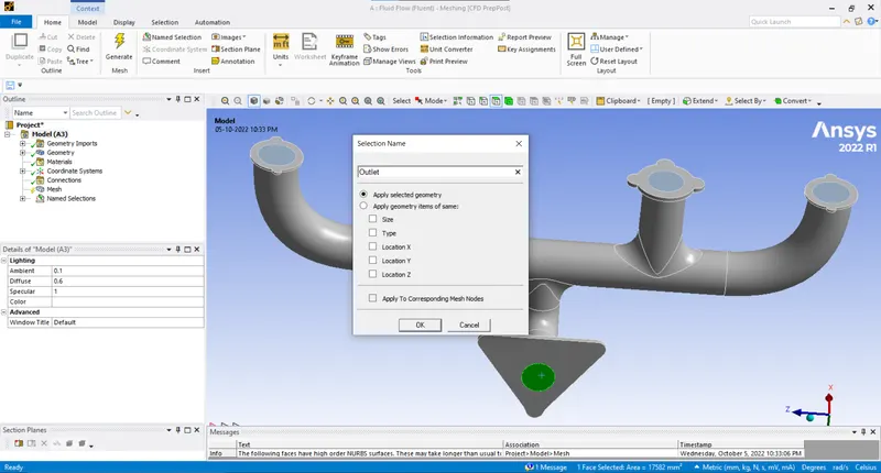
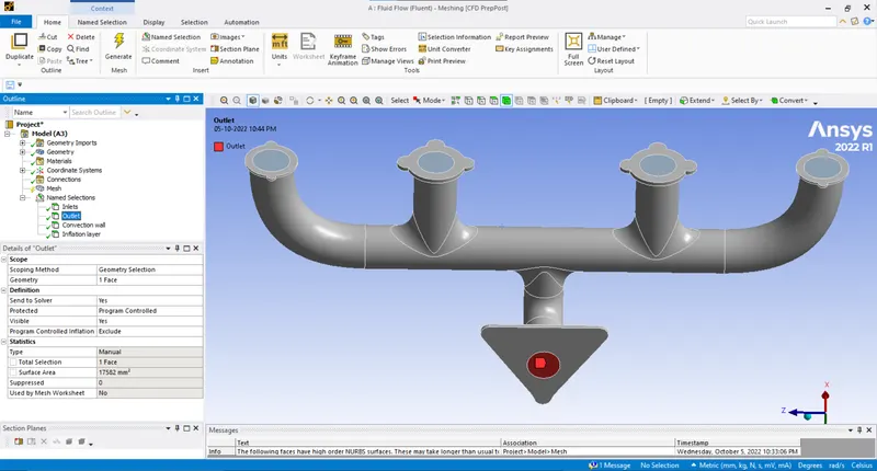
- Outlet:
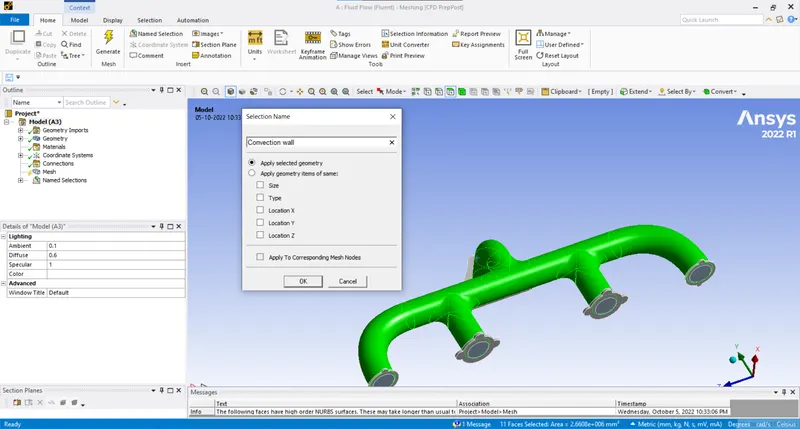
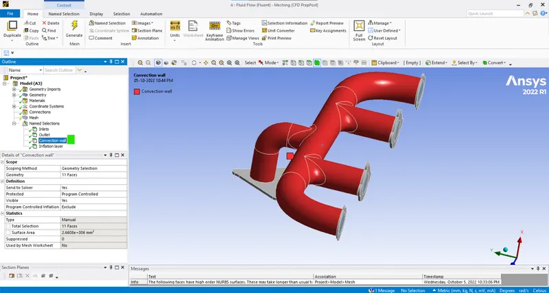
- Convection wall:
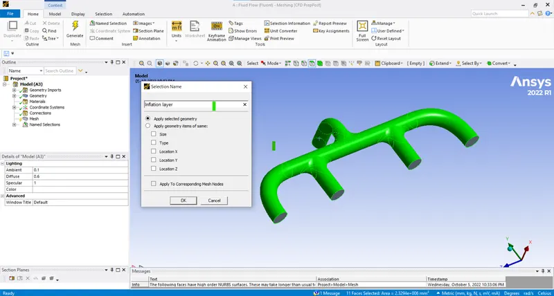
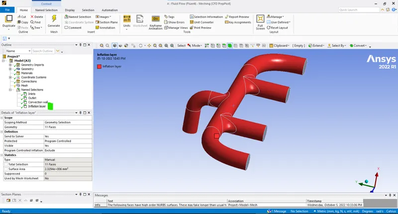
- Inflation layers:
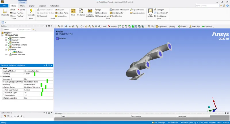
- Now as the naming is complete we can proceed to providing inflation layers and meshing the whole geometry (Mesh > Insert > Inflation layers):
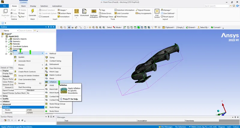
- Method by named selections > Inflations:
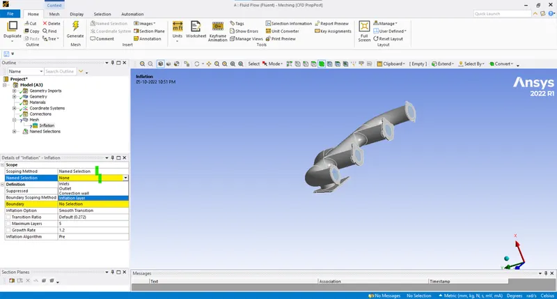
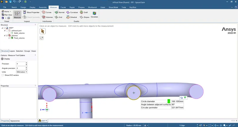
- Characteristic length = 166.109mm
- Calculation the y+:
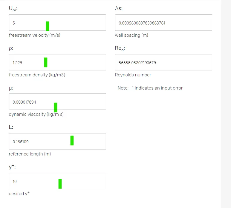
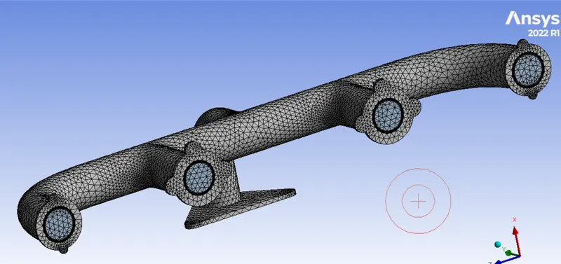
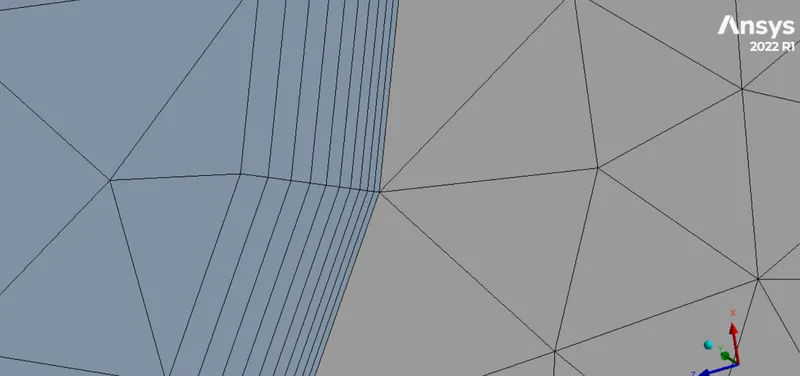
- Initial cell count (150mm):
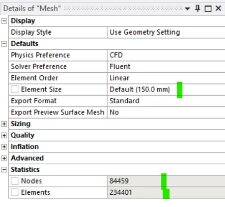
- Update the mesh (Mesh > Right click > Update):
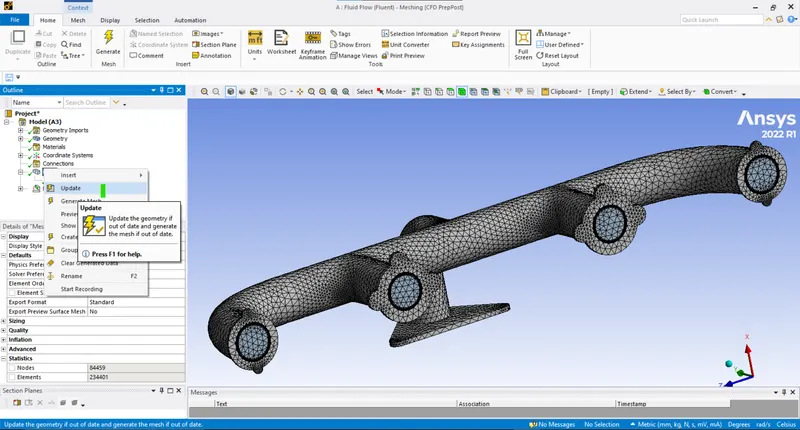
- Now the meshing is complete we can proceed to the setup.
- Setup (Right click > Setup > Edit):
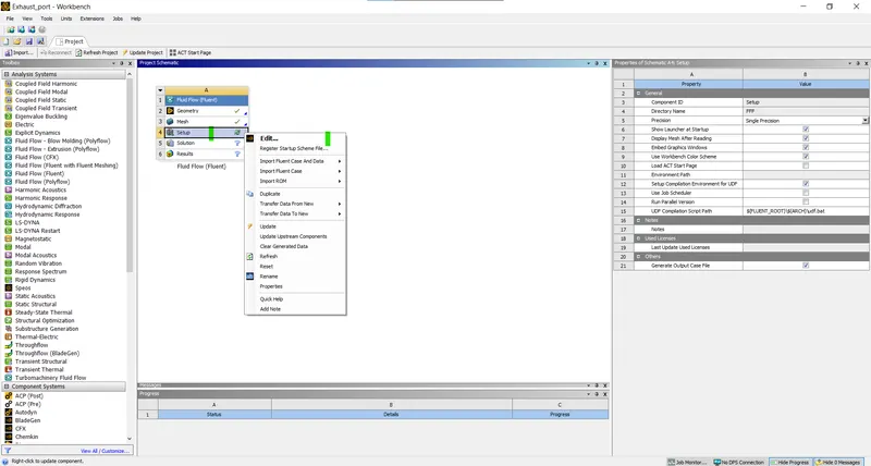
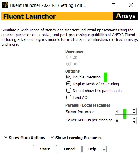
- Set the double precision and appropriate number of cores.
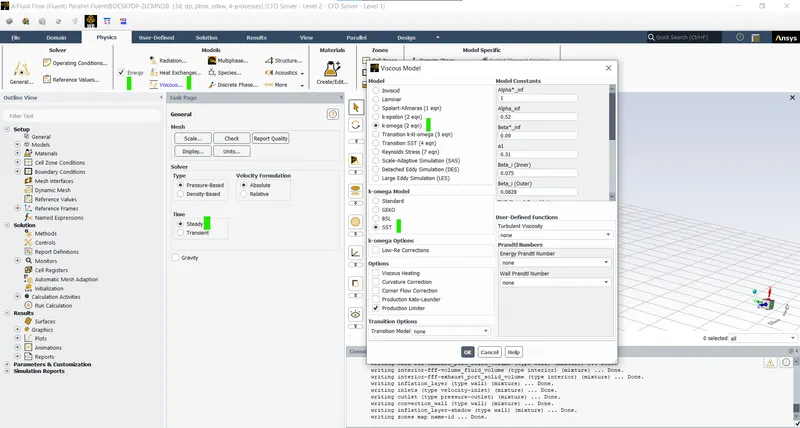
- Selecting the steady state and viscous model as k-omega (SST) model with energy equation is on:
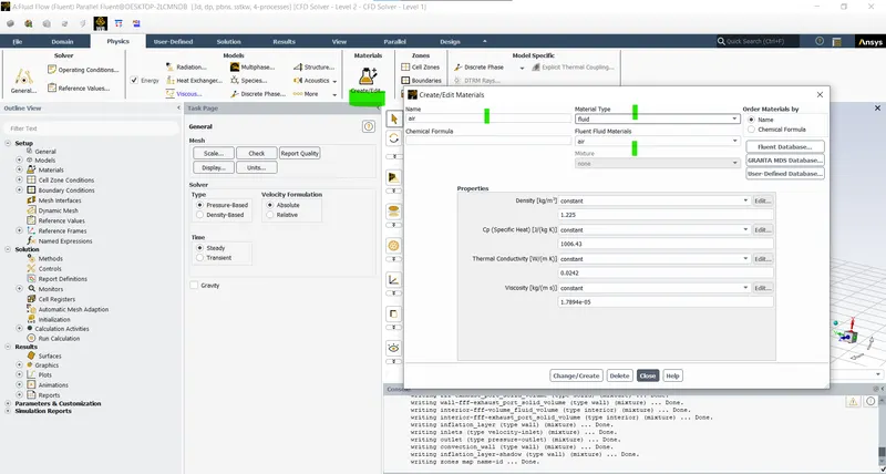
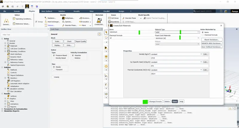
- Selecting the materials:
- Air (Fluid > Air):
- Aluminium (select solid > Aluminium):
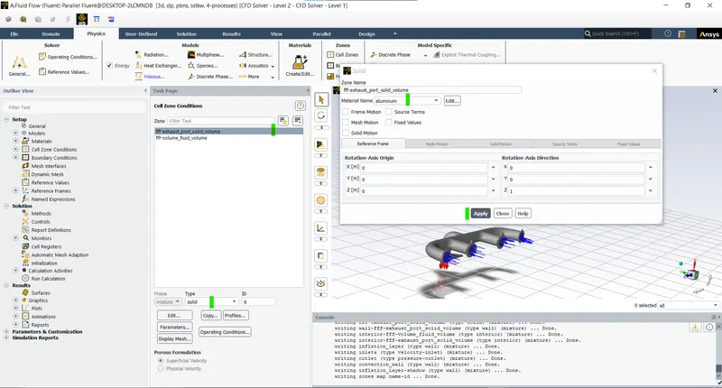
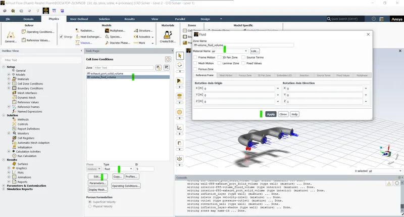
- Assigining the materials to the cell zones.
- Solid material - Aluminum:
- Fluid volume - Air:
- Defining the boundary conditions:
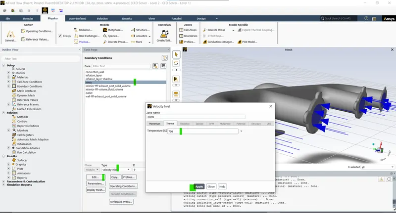
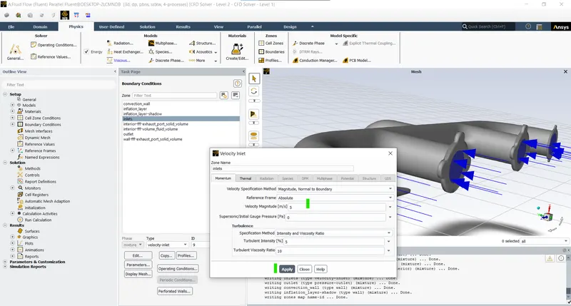
- Inlet (velocity inlet):
- Velocity at the inlet is 5m/s amd the temperature is 700k.
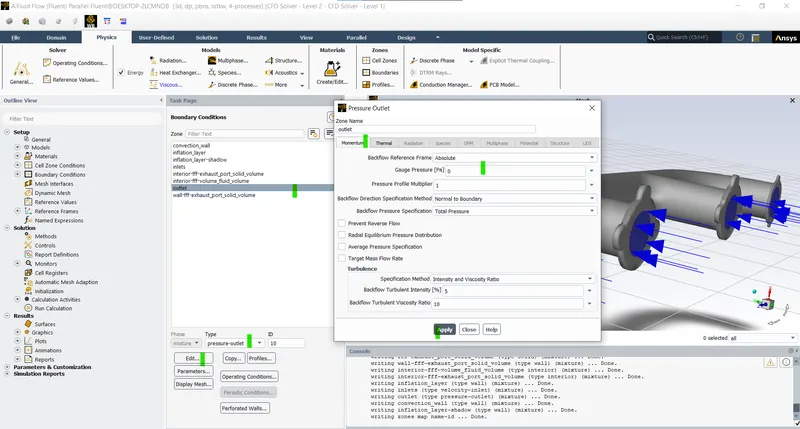
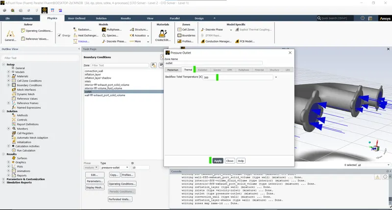
- Outlet (Pressure outlet):
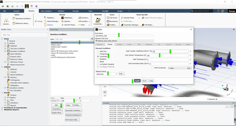
- Convection wall (convection - 20W/(m^2)k):
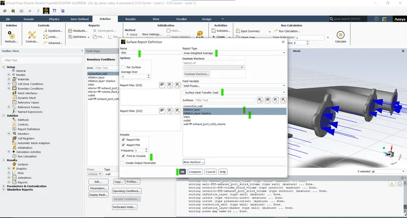
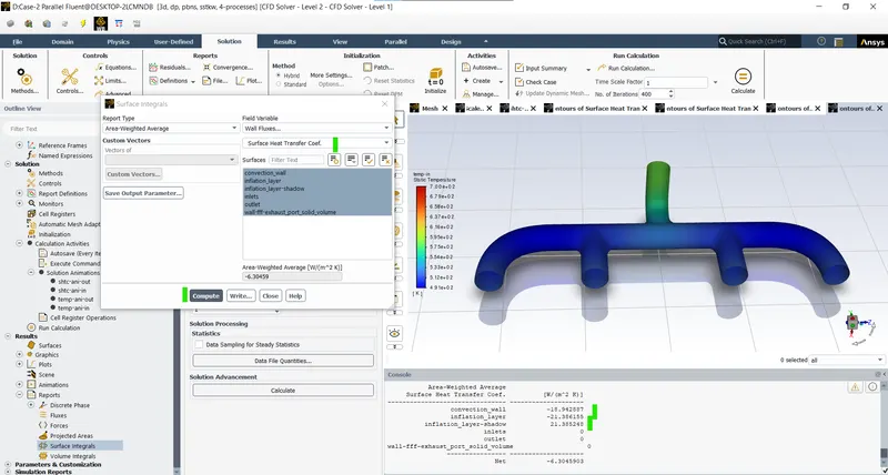
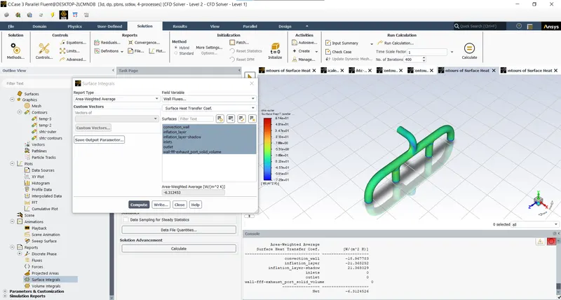
- Defining the report definitions (Solutions > Definitions > Area weighted average > Wall fluxes > Surface heat transfer co-efficient at inflation layer > Ok):
- Surface heat transfer co-efficients:
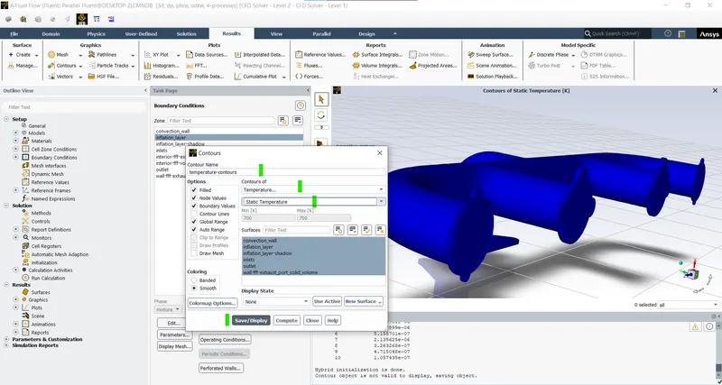
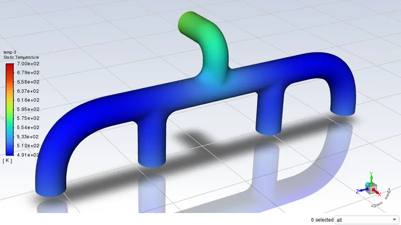
- Now creating the contours for visulaization (Initialize > Contours > Temperature > External/ all components > Ok):
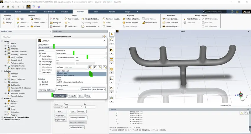
- Surface heat transfer co-efficient at inflation layers:
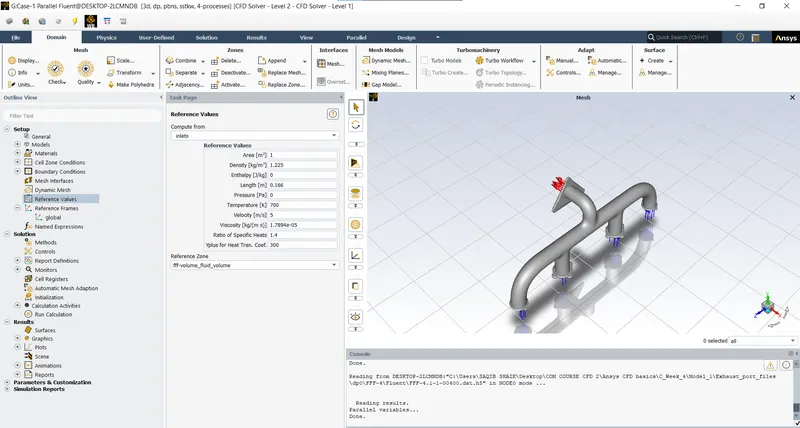
- Computing from inlet (Reference values > select compute from inlet > set length):
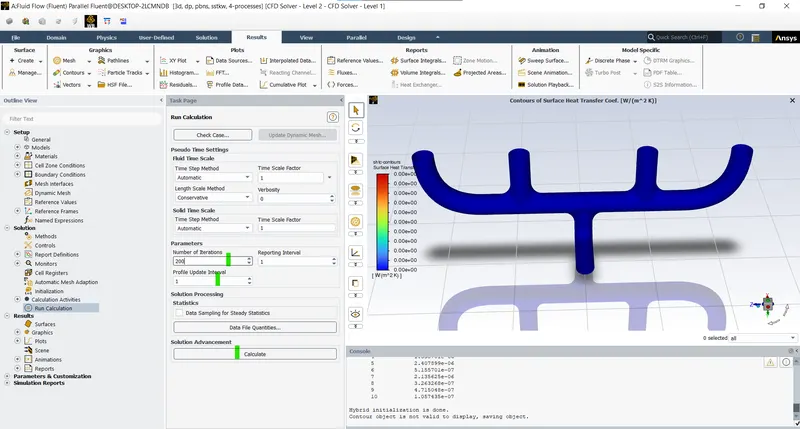
- Running the calculations for 200 iterations while saving the data at every iterations:\
- Now computing the surface heat transfer co-efficient at inflation layer (Surface reports > Area weighted average > Wall fluxes/Temperature > Surface heat transfer co-efficient/Static Temperrature):
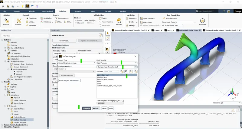
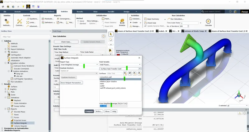
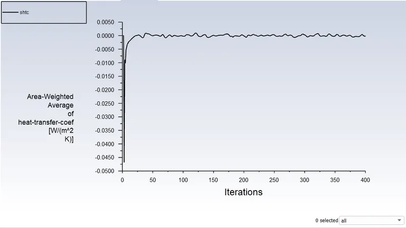
- Surface heat transfer co-efficient = -21.3949 W/m2k.
- Temperature at outlet = 677.4414k.
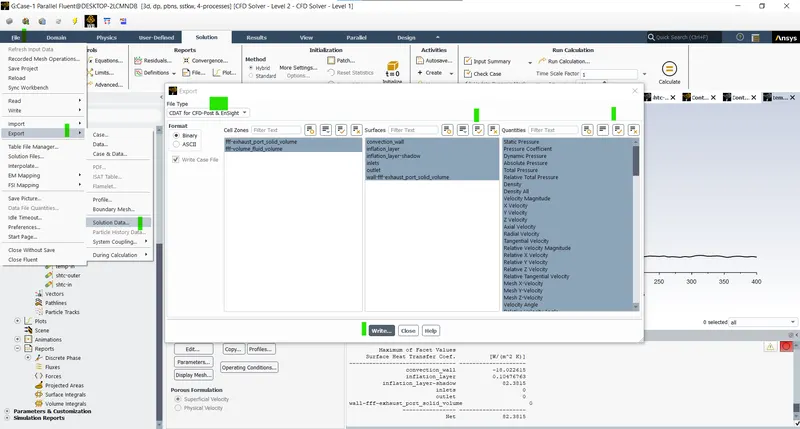
- As we need to have the wall flux data in the post processing we need to export the CDAT file containing the useful information to post processing (File > Export > Solution > CDAT format > select information > Write):
- After soving we need to check the yplus value near the wall (Surface reports > Area weighted average > Turbulence > Wall yplus > Select the region > Ok):
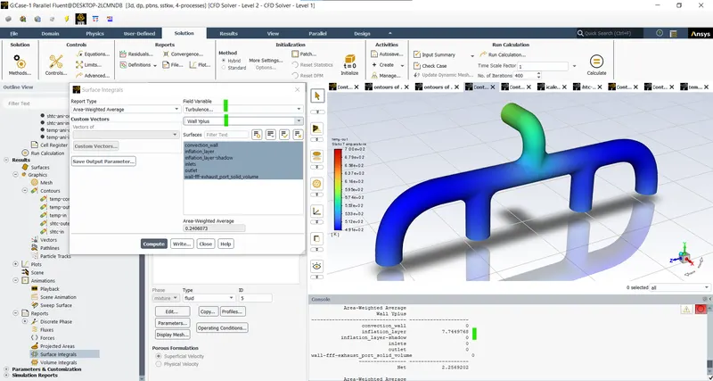 \
\- Initially we assumed the standard value for the yplus for k-omega SST model and after calculation we reasses the value and find find the new y-distance.
- `y ^+ = (y u )/ ν`
- where y = distance of the first cell/First cell thickness.
- u = Free stream velocity.
- v = Kinematic viscosity.
- We need to calculate the y-distance as we all the other values and proceed.
- New yplus is 0.4mm.
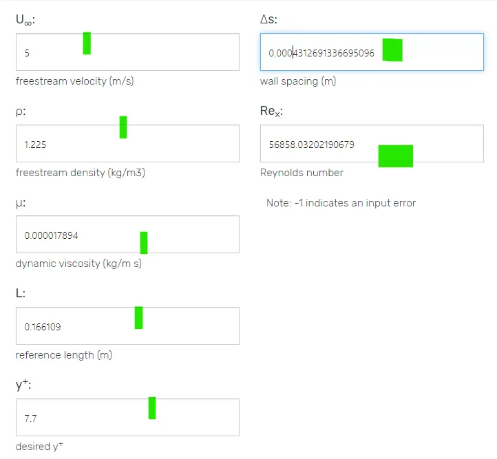
- Remodelling the geometry in the mesh and calculating it once again with actual y-plus.
- Now we can import this information as results in the post processing by import results in the file options.
- Post-processing (Results > Right click > Ok):
- Temperature profiles nar the outlet:
- Insert the plane in the xy plane (Insert > Location > Plane > Rename > Select the xy plane > Color > Variable > Temperature):
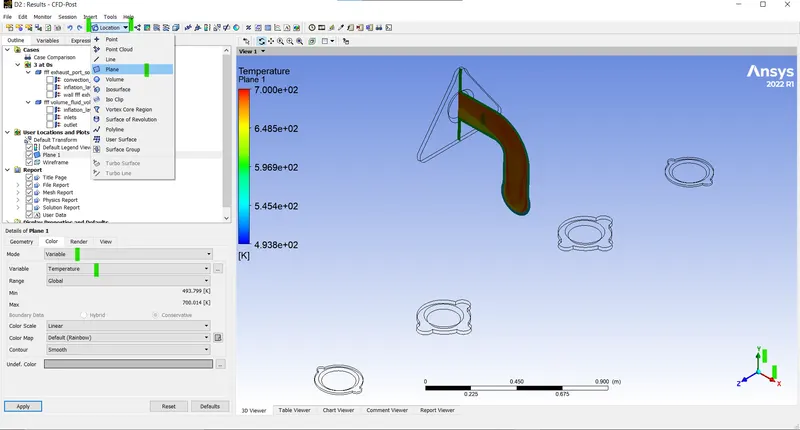
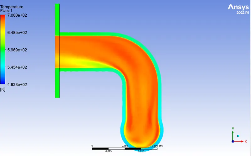
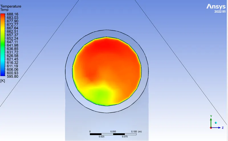
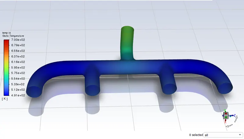
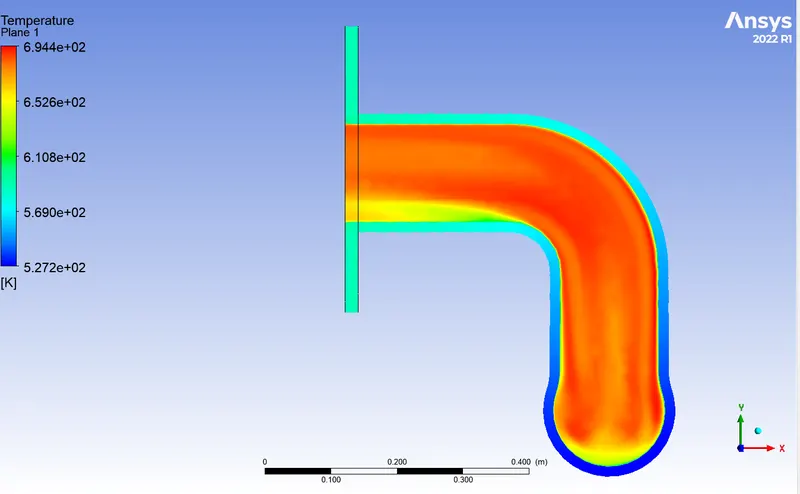
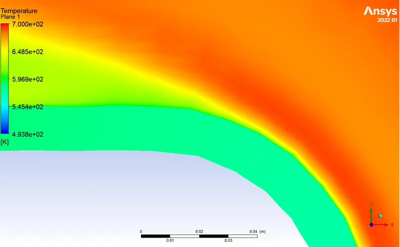
- The figure represents the temperature contours near the outlet of the exhaust it can be seen that due to aluminum having high thermal conductivity the heat near the solid region dissipates more quickly compared to the inner convection hence we can see that there low temperature zone at the solid fluid interface.
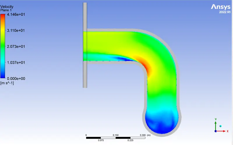
- Now same procedure for velocity:
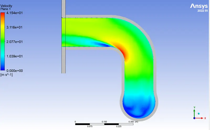
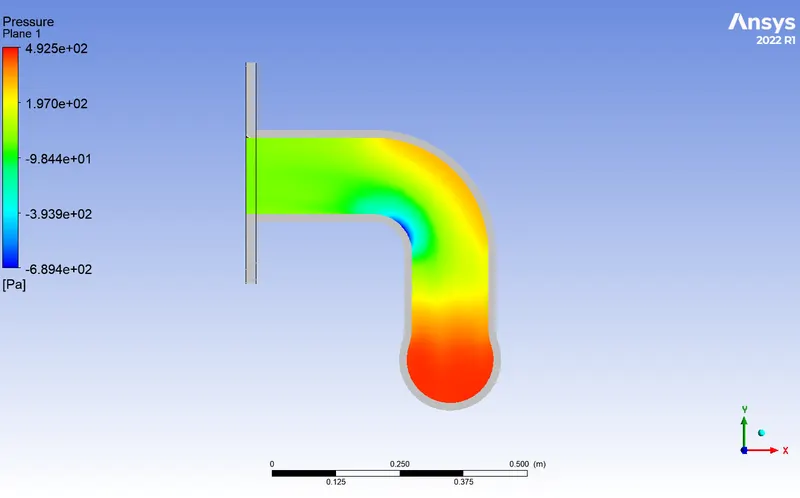
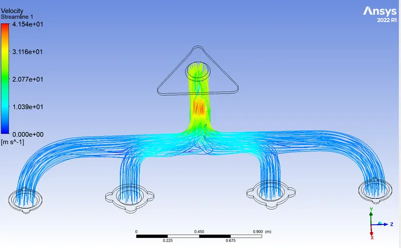
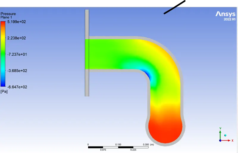
- It can be seen that due to the curvature near the exhaust outlet there is change in velocity as when it enters the exhaust outlet pipe the velocity increases as there is a contraction and mass flow from the each inlet add up and at the bent there is change in velocity as the momentum pushes the fluid in the stright path and and so the pressure at the outter curve of the inflation and the area shown in the red contours means it has very less pressure and hence the velocity will be high and as the flow just passes the bent the there is area of very less velocity, the whole process of velocity change is due to the massflow adding up and the curvature at the exhaust which can be observed from the pressure and velocity contours.
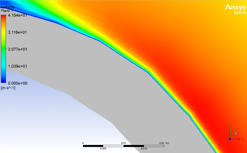
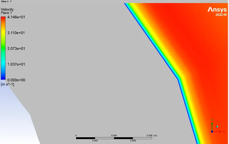
- Here the no slip condition near the boundary is clearly visible
- Now for the pressure contours:
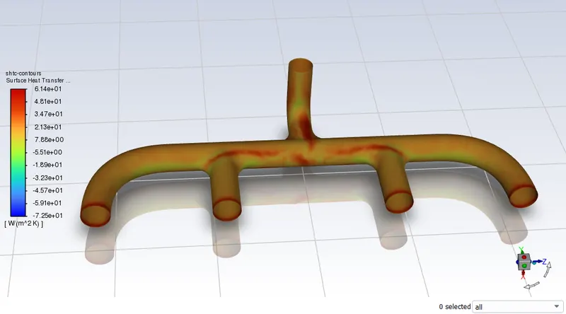
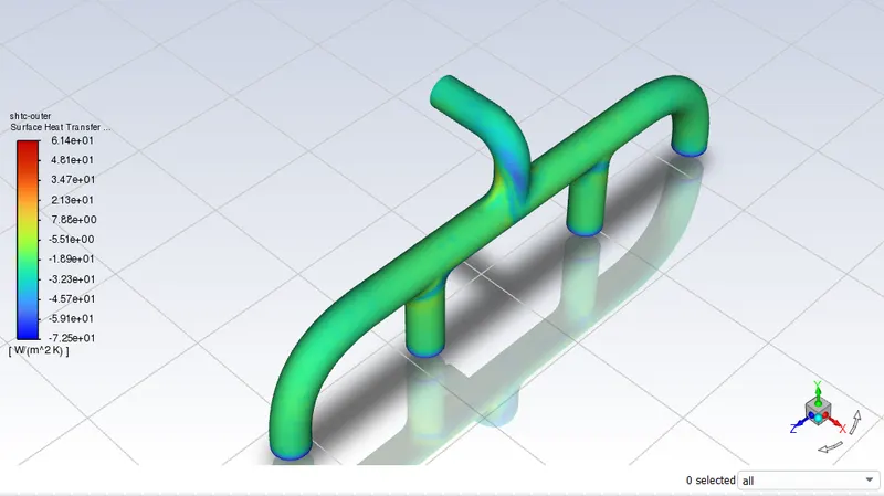
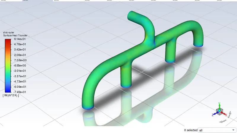
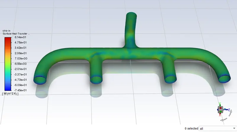
- Now for surface heat trnasfer co-efficient:
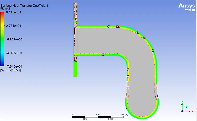
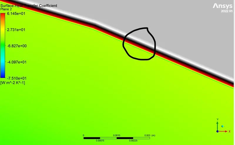
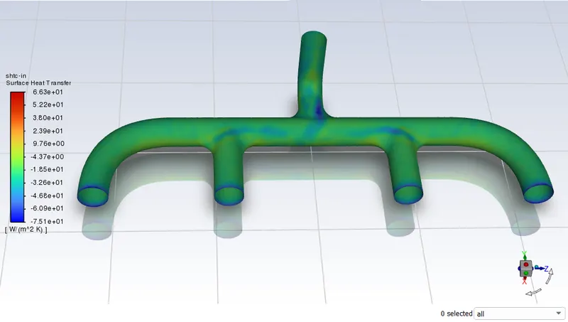
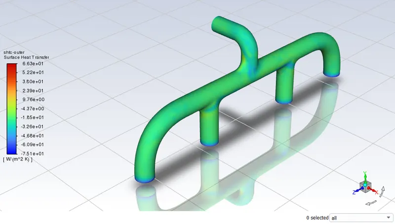
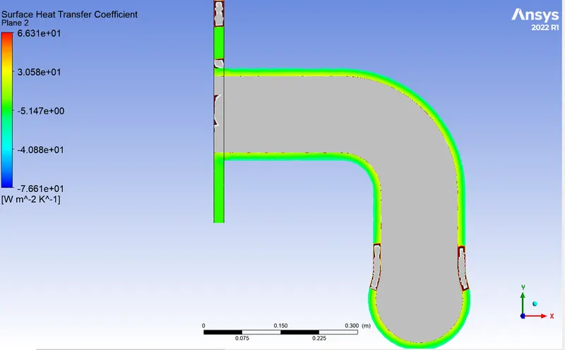
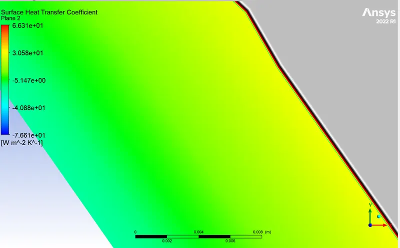
- It can be seen that as there is hot air inside the exhaust the surface heat transfer co-efficient is higher near the inside wall and as it moves outward it reduces as the temperature difference/gradient is decreasing.
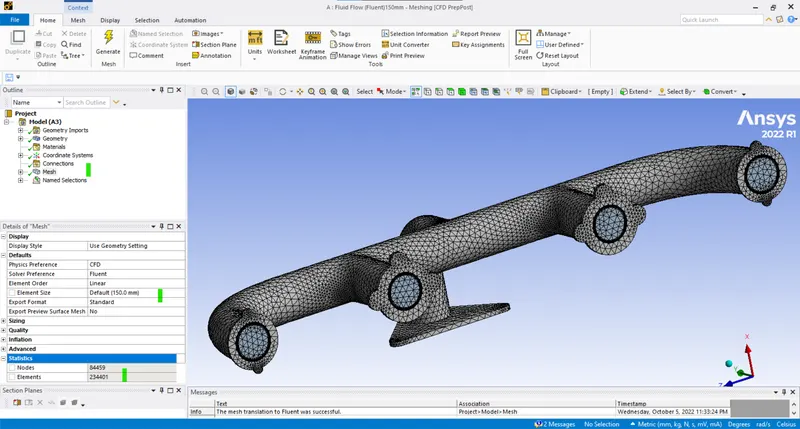
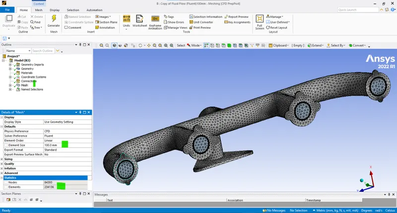
- Now checking the mesh independency on the geometry mesh:
- Case-2:
- Element size = 75mm.
- Inflation layers = 0.5mm thickness, 15 layers.
- Face sizing = 25mm.
- Body sizing = 25mm.
- Number of elements = 230906.
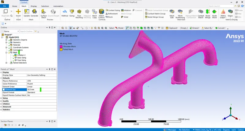
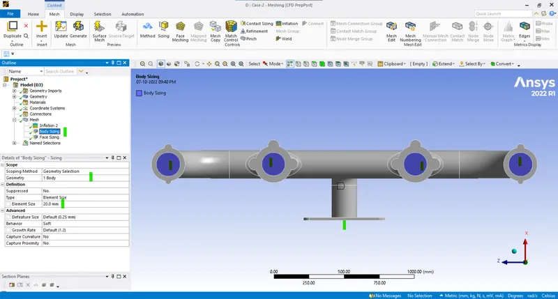
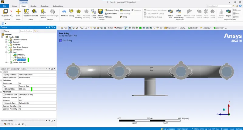
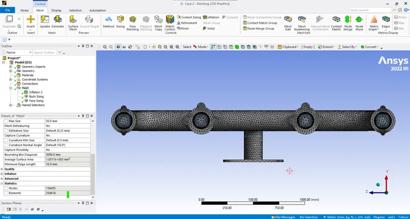
- Case-2:
- Element size = 50mm.
- Inflation layers = 0.5mm thickness, 15 layers.
- Face sizing = 20mm.
- Body sizing = 20mm.
- Number of elements = 334618.
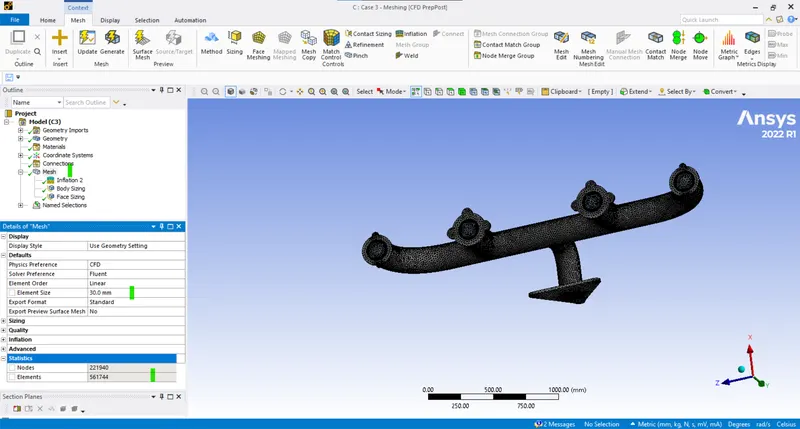
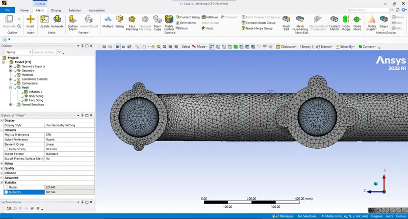
- Case-3:
- Element size 30mm.
- Inflation layers = 0.5mm thickness, 15 layers.
- Body sizing = 15mm.
- Face sizing = 15mm.
- Cell count = 561744.
- Case-2:
Results:
- Case-1:
- Mesh count: 230906.
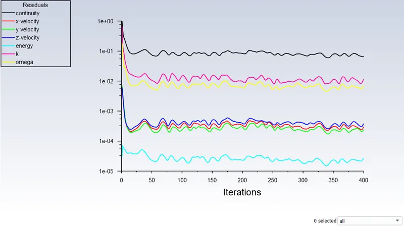
- Residuals:
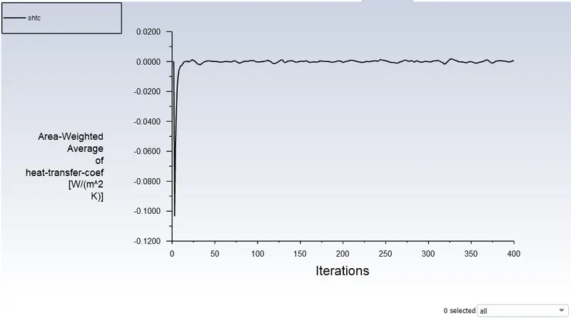
- Surface heat transfer co-efficient:
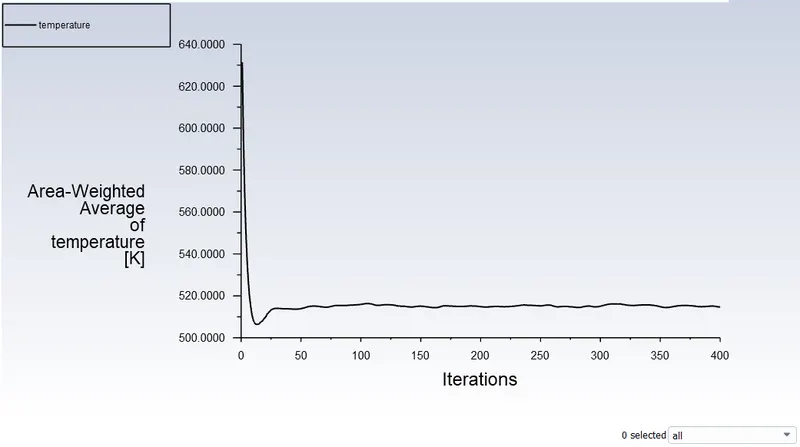
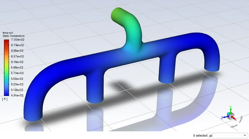
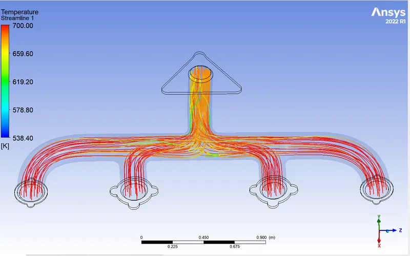
- Temperature:
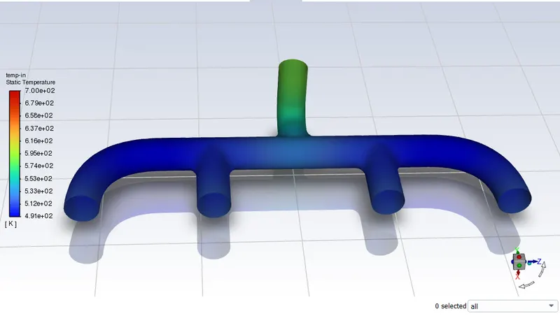
- At outlet:
- Velocity:
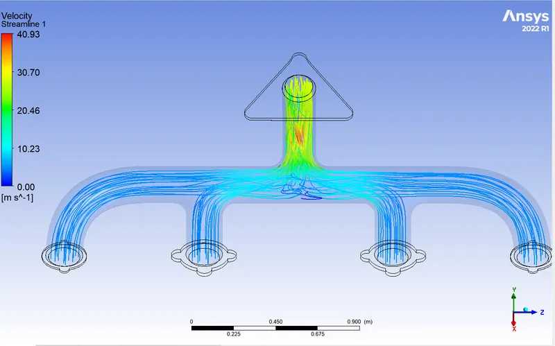
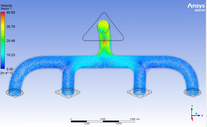
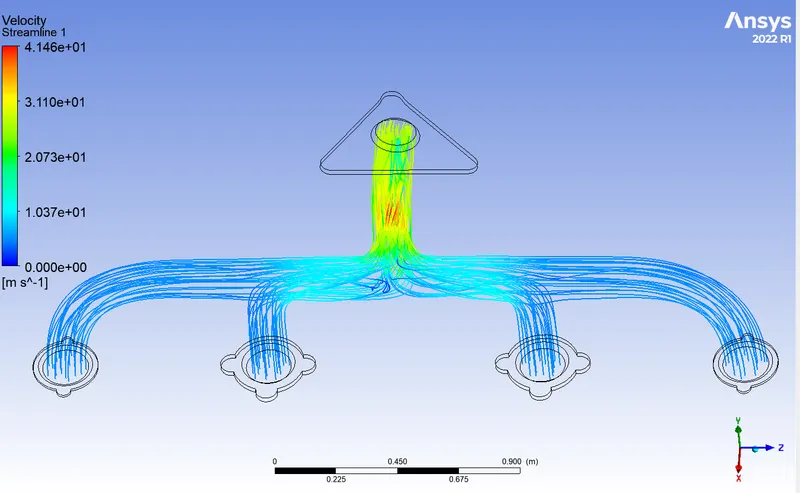
- As we can see at the at the sections were the tubes combine there is increment in the velocity as the mass input and mass output must be conserved.
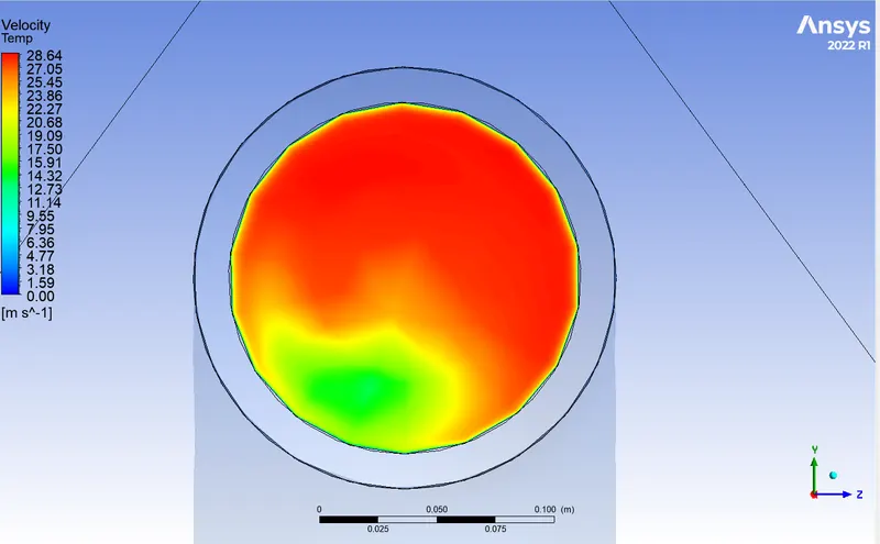
- At outlet
- Case-2:
- Mesh count: 334618.
- Residuals:
- Surface heat transfer co-efficient:
- At outlet:
- Temperature:
- At outlet:
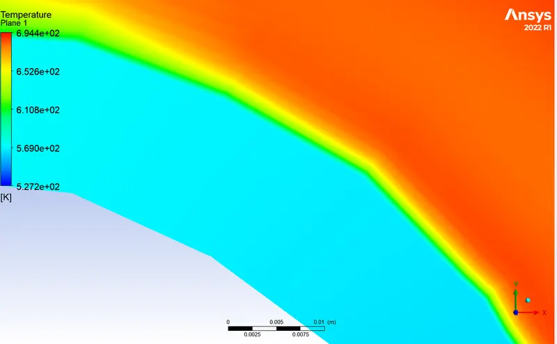
- Pressure:
- Velocity:
- Case-3:
- Residuals:
- Surface heat transfer co-efficient:
- At outlet:
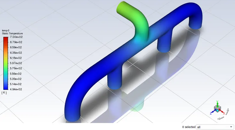
- Temperature:
- At Outlet:
- Velocity:
- Near the outlet:
- Pressure:
- Near outlet:
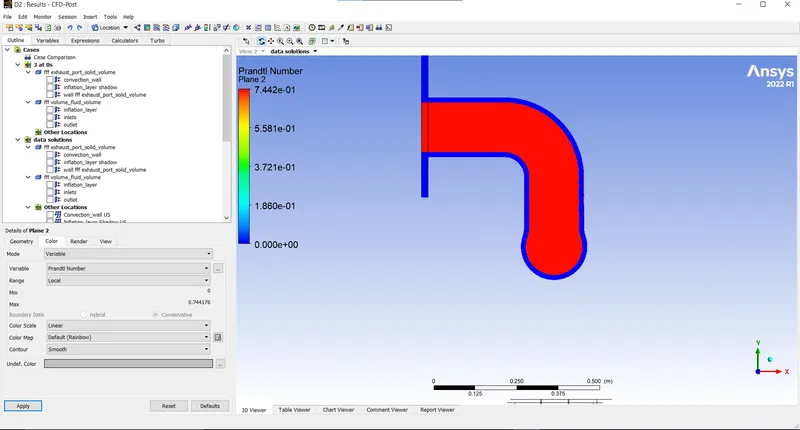
- Prandtl Number:
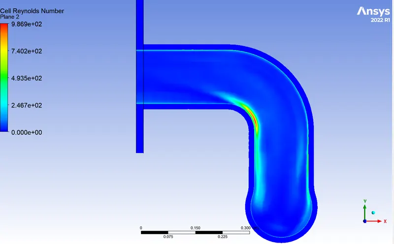
- Cell Reynolds Number:
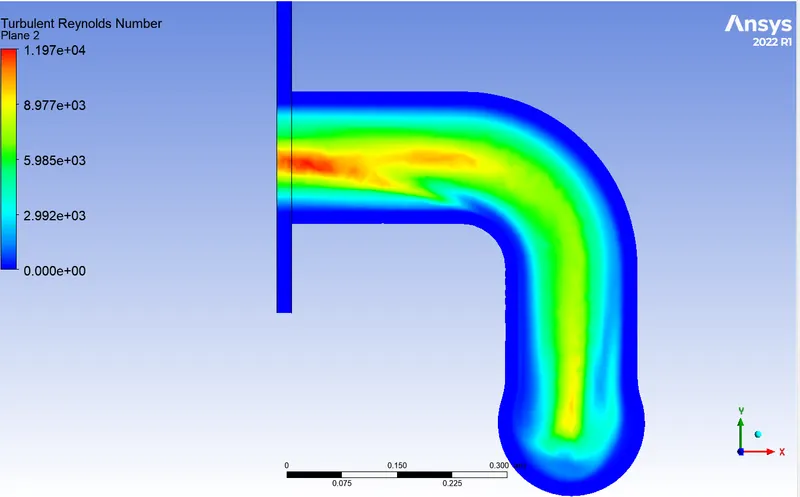
- Turbulent Reynolds Number:
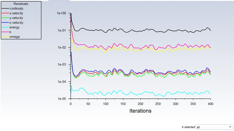
- Residuals:
- Theoretical calculation:
- Nusselt Number: Here as the flow is internal and inside the bent tube we can have this corelation for Nusselt number in terms of Reynolds number and Prandtl number:
- `Nu = 0.023*(Re)^(4/5)*(Pr)^(0.3)`
- Where Re = Reynolds number = `(rho*v*D)/(mu)`
- Pr = Prandtl Number which can be found out using the Heat transfer corelation from data book.
- Nusselt number = `(h*D)/k`
- `rho`= Density of the fluid `(kg)/(m^3)`
- `v`= Velocity of the fluid `(m/sec)`
- D = Characteristic length (Diameter) (m).
- `mu`= Dynamic viscosity `(kg)/(ms)`.
- h = Convective heat transfer co-efficient `(W)/(m^2*k)`.
- k = Thermal conductivity `(W)/(m^2*k)`
- Re = (1.225*5*0.166)/(0.000017894) = 56821.
- Pr = 0.684 at 700 kelvin.
- Nu = `0.023*(56821)^(4/5)*(0.684)^0.3` = 130.57
- `= (0.0242*130.57)/(0.166) = 19.03 W/(m^2k)`
- Content table:
-
Number of elements Mass Flux (kg/s) Inlet Velocity (m/s) SHTC (Numerical) SHTC (Therotical) Temp (k) (out) Case-1 230906 0.53752477 5 21.35 19.03 677.893 Case-2 334618 0.53908877 5 21.385 19.03 677.89394 Case-3 561744 0.54074969 5 21.368 19.03 677.85153 - The error between the therotical and the numerical surface heat transfer coefficient is around 10% which is due to the reasons that we have the correlation if the stright pipe internal flow but the exhaust pipe has many curves and bents at varying cross-section which leaves the correlations not so accurate as to the fit the geometry and flow conditions.
-
- Animation table:
-
Cases SHTC Temperature Velocity Case-1 Velocity streamline Case-2 SHTC Temperature Velocity streamline Case-3 Temperature Velocity streamline
-
1. Give a brief description of why and where a CHT analysis is used.
- The conjugate heat transfer or CHT analysis is used were there is heat transfer between the solid and the fluid i.e. were both conduction and convection occurs to study the rate of heat transfer as the time proceeds.
- It is used were heat transfer coefficient change as the function of of temperature.
- CHT is used to simulate the behaviour of heat transfer within and between the fluid and solid.
- It can be very helpful predicting the outcome of the case understudy with much improved than assigning as constant heat transfer co-efficient.
- The applications were CHT is applied is very broad some of the examples are given below:
- Turbocharger.
- Heat engines.
- Cryogenics.
- Heat exchangers.
- HVAC.
- Combustion chambers.
- Furnace.
- Microprocessors.
- Battery mangament/assesment system.
- Basically in all the cases were the conduction and convection occurs simultaniously (i.e. were the heat is transfered between solid and fluid).
2. How would you verify if the HTC predictions from the simulations are right? On what factors does the accuracy of the prediction depend on?
- The analysis results are validated by using the theoretical correlations and the results fall within the acceptance range.
- The accuracy of the simulation prediction depends on the following factors:
- Selecting the appropriate viscous model.
- Y plus value.
- Refinement of the mesh.
- On realistic boundary conditions (How close we are able define the boundary condtions compare to the realistic conditions).
Conclusions:
- The conjugate heat transfer simulation is run successfully for the given geomety after cleaning and properly meshing the gemetry.
- The results are analysed and presented in the form of this report.
- The numerical simulation is validated with the theoretical calculations.
- Three cases are run to conform the study is independent of the mesh properties.
- The mesh independency is achived with accuracy of one digit after decimal.
- The surface heat transfer co-efficient at the inner side of the solid is 21.3 `W/(m^2k)` and the theoretical values are 19.03 `W/(m^2k)`