Week 3 - External flow simulation over an Ahmed body.
Aim: To run the aerodynamic study on the Ahmed Body using the symmetrical half of the body and run the grid independency test to ensure the results are accurate.
Objective:
- Import the geometry into spaceclaim.
- Design the enclosures ensuring no interfering volumes.
- Split the geometry into symmetrical half.
- Perform Grid Independency test(0.3, 0.5, 1 million cells).
- Perform the simulation.
- Analyse the wake region and point of seperation.
- Conclude the results analysed.
Theory:
- Ahmed Body:
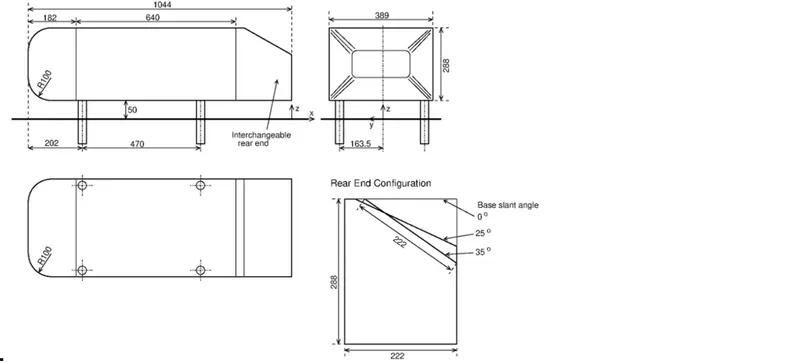
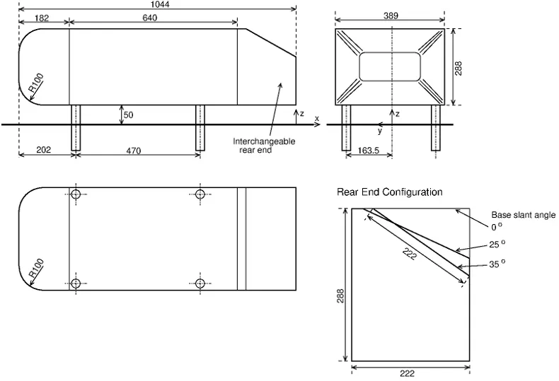
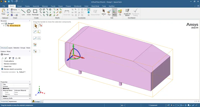
- Created by S.R. AHMED in 1984 for the study of the study the Salient feature of Time-average wake on the vehicle body the Ahmed body became the benchmarking model for validating the numerical aerodynamic simulation of the vehicle model.
- It represents basic passenger car with the length of 1.033m, width of 0.389 and height of 0.288.
- The study performed on this generic car model were experimental and depects the generic senario of the car, this gives us very important standard benchmark to compare and validate the numerical aerodynamic study done.
Content of the Body:
- Import the Ahmed Body into the Ansys Fluent in Ansys Workbench (Drag and drop).
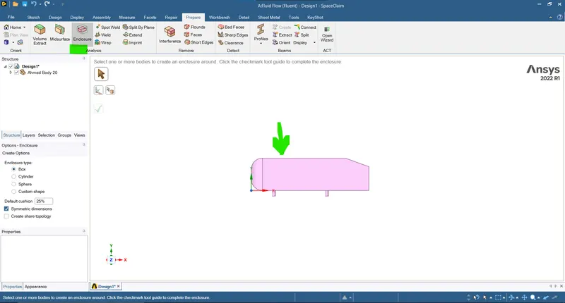
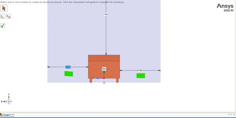
- Now we need to create the enclosure to cover the Ahmed Body representing the area used for the simulation around the Ahmed Body (Prepare > Enclosure > select the Ahmed Body > give the dimensions):
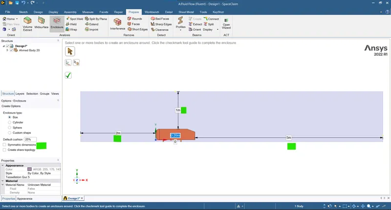
- Give the dimensions:
- Error:
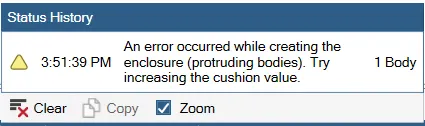
- This error is caused due to the 0 mm enclosure below the Ahmed Body.
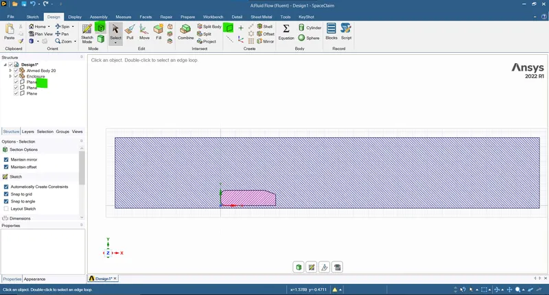
- Now create the section plane to view the cross section of the enclosure and Ahmed Body (Planes > Select the desired plane > click on the section view) :
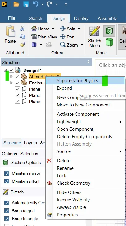
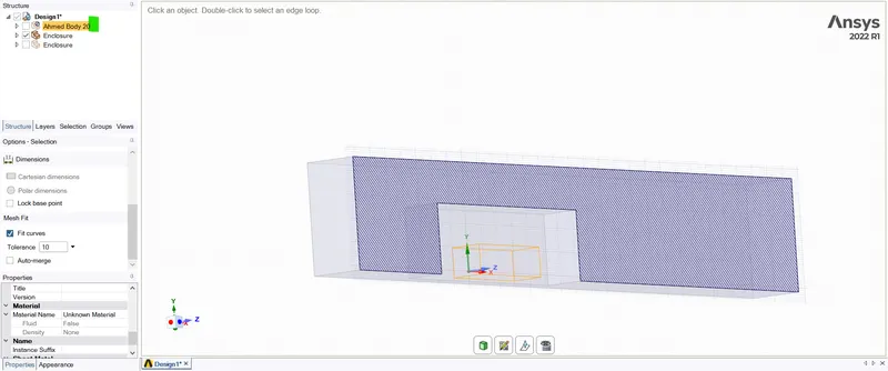
- Now as we are considering the aerodynamic simulation outside the body we can suppress the Ahmed Body for physics so it's not used in the computaion during the simuulation (Right click on the Ahmed Body > Suppress for Physics):
- As we are more conserned towards the flow near the walls, so to refine the mesh in the near wall/body we are going to create another enclosure and delete the interfaces and go for meshing:
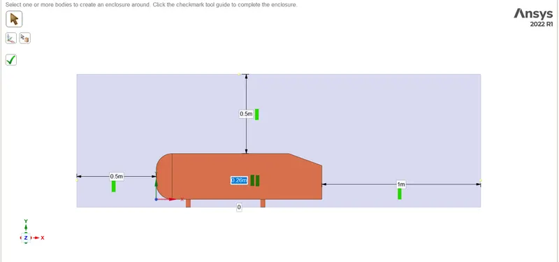
- Giving the dimensions to second enclosure:
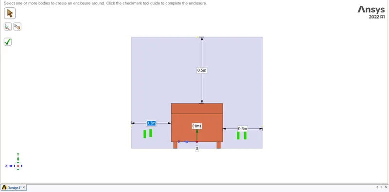
- Now viewing the cross section:
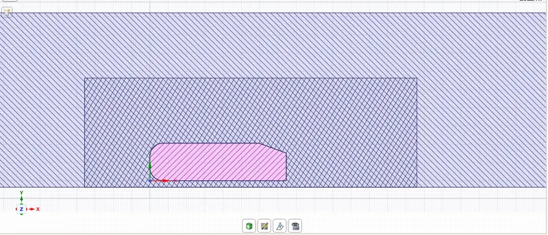
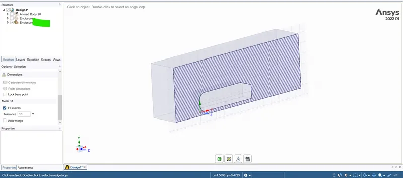
- As we can see the double cross section the two enclosure intersecting regions, we have to delete the first enclosure volume which is intersecting with the second enclosure using the inteference command (Interference > select the geometry > click Ok):
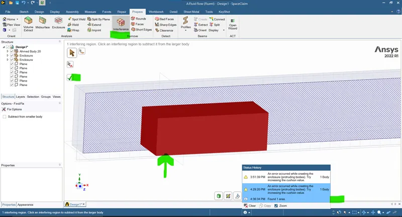
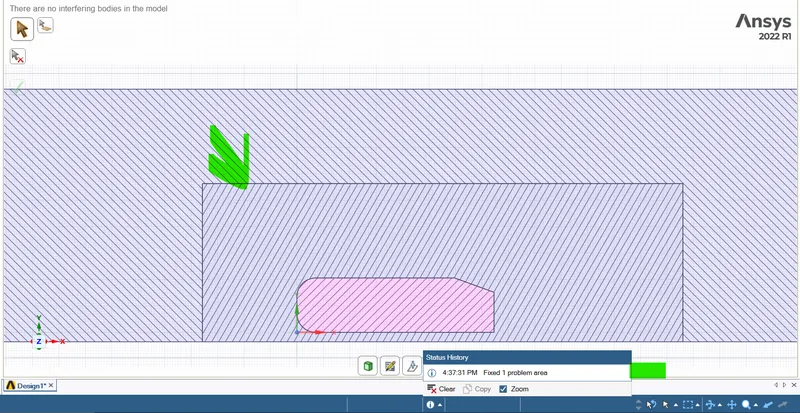
- The interference is cleared as seen the cross hatches are in singular lining.
- Enclosure-1:
- Enclosure-2:
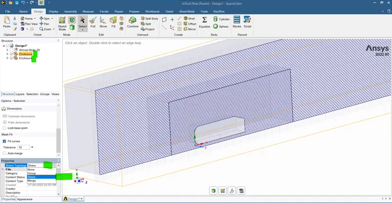
- Topology must be shared in order to transfer the computed data between the Enclosures (Select the Enclosure > Share Topology > Shared) :
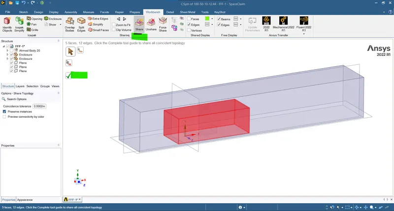
- Now sharing the parameters:
- Now as the geometry is perfectly symmetrical we can split the body and run the simulation on the one half:
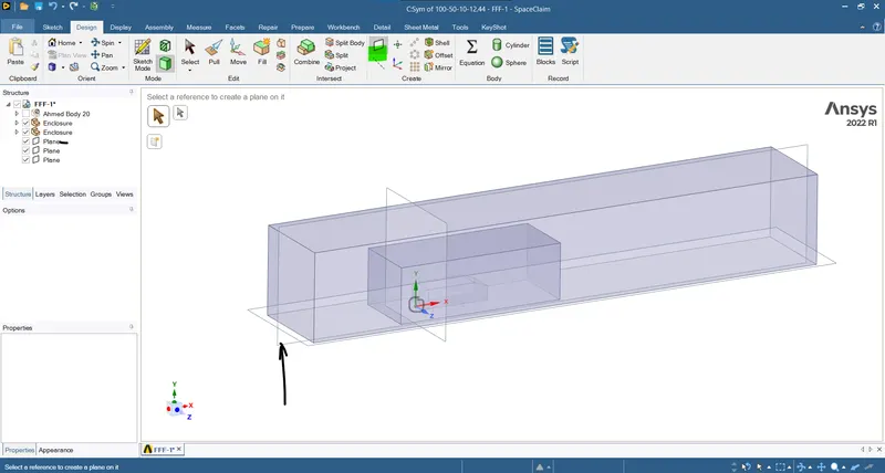
- First creeating the section plane to disect the symmetry (In xy plane):
- Using the split body command first select the body and the plane then the body to be deleted:
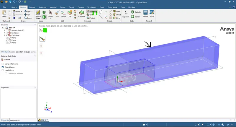
- Cut plane:
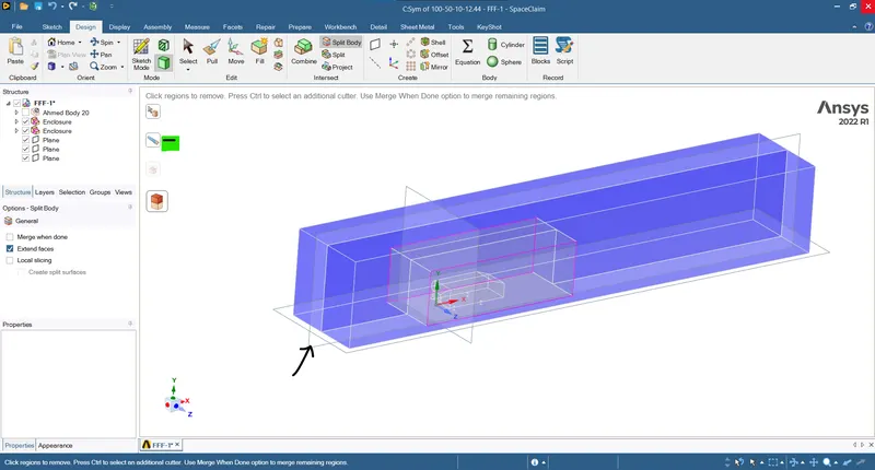
- Body to be deleted:
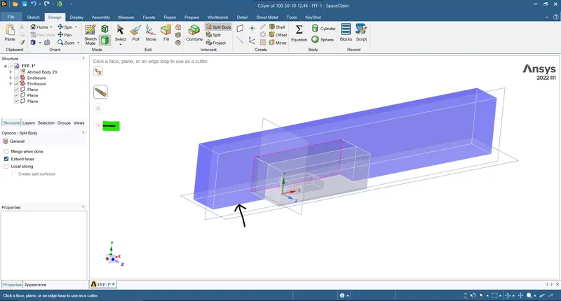
- Repeat the process for inner enclosure and the Ahmed Body:
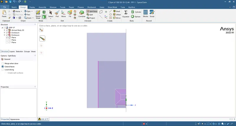
- Now as the geometry is ready we can now proceed to the meshing part:
- Now open the mesh in the Ansys Fluent tool and generate the default mesh (Mesh > Generate Mesh):
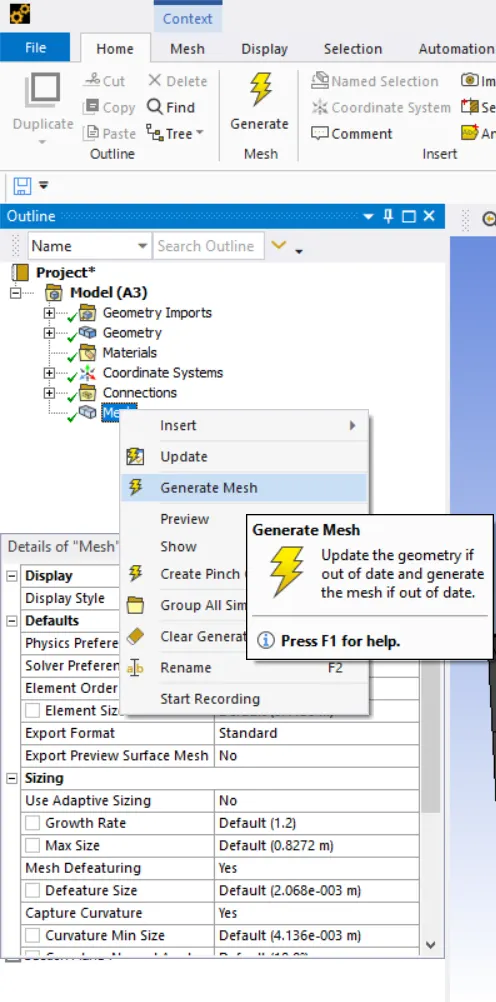
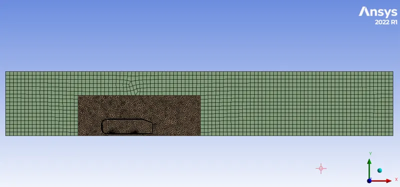
- Initially the default generated mesh is very coarse and the contours and other useful parameter will not be properly depicted:
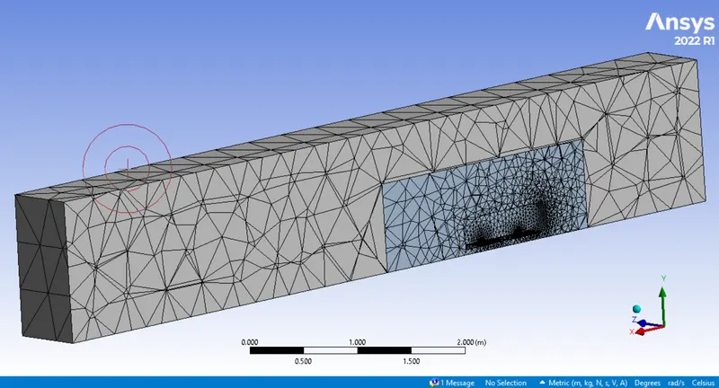
- So we need to refine the mesh:
- Firstly as the outer volume is mostly square in shape we will change the mesh type from tetrahedrun to Hexahedron (Mesh > Insert > Method > Multizone):
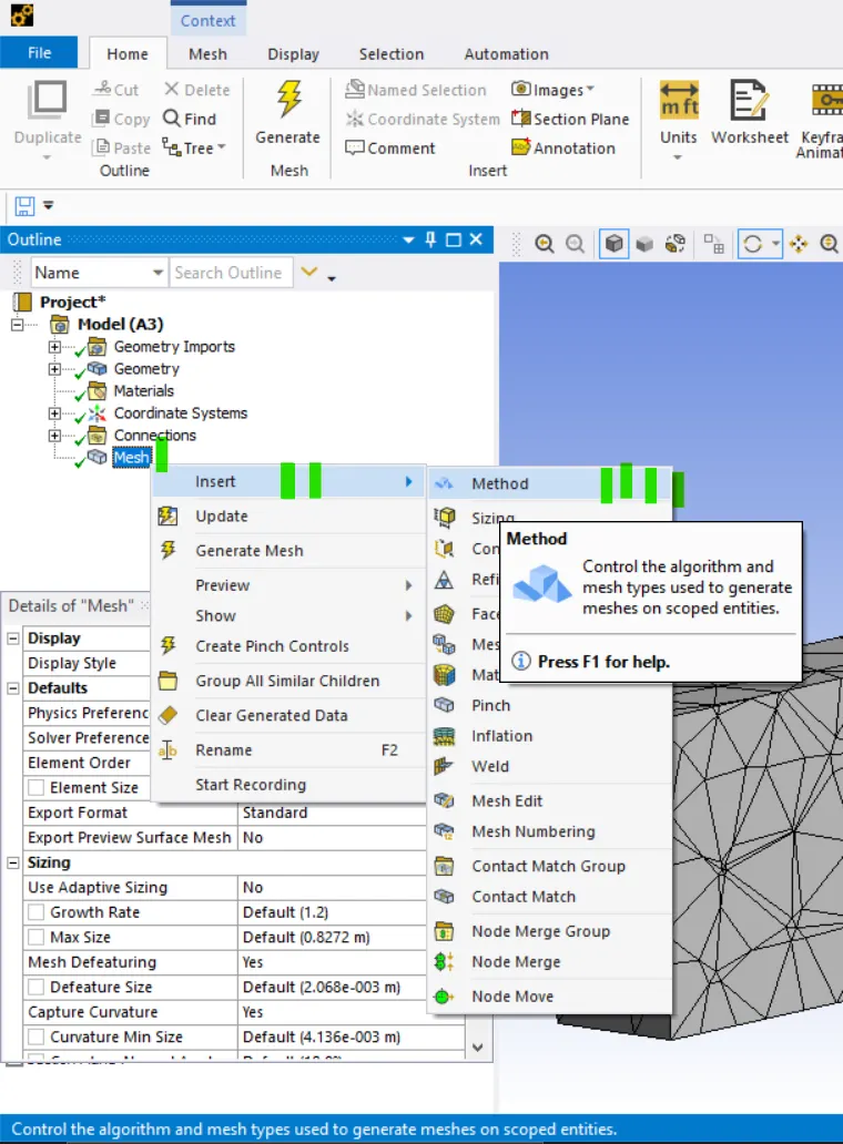
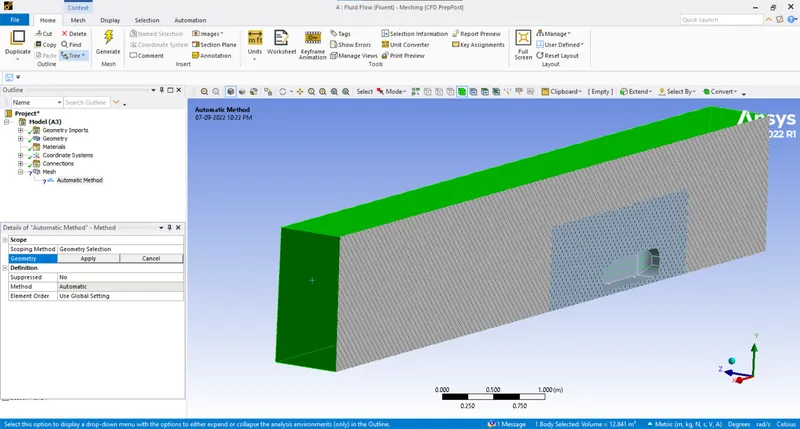
- Selecting the body for the method:
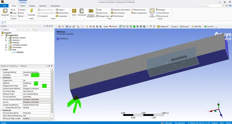
- Selecting the multizone method as it will generate mostly the hexahedron mesh were ever neccessary and rest of the case it generates the default mesh:
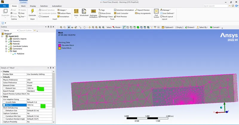
- Now defining the element size as 100 mm the default section of the mesh and defining the maximum size to be 100 mm as to attain the uniform element length:
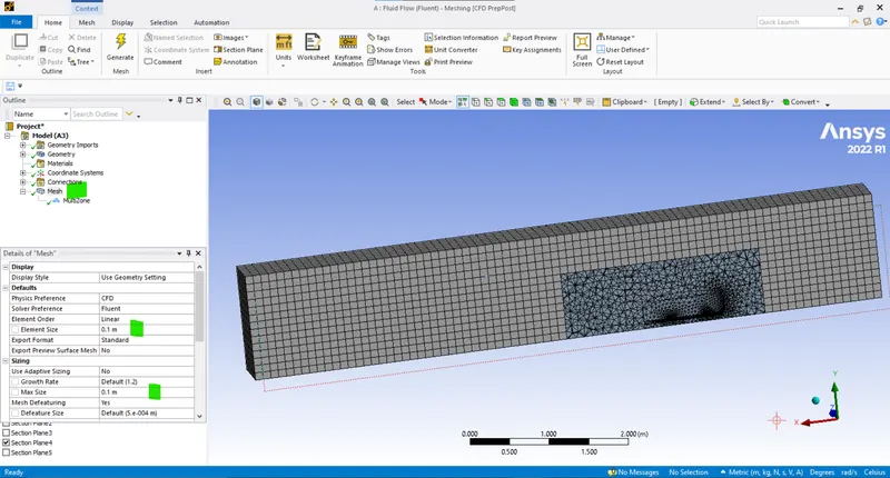
- After defining for 10 mm and updating the mesh:
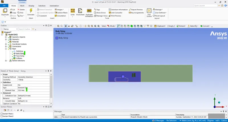
- Now refining the mesh near the Ahmed body(50 mm):
- Insert the sizing method for the enclosure (Mesh > Insert > sizing > select the body > define the size > ok):
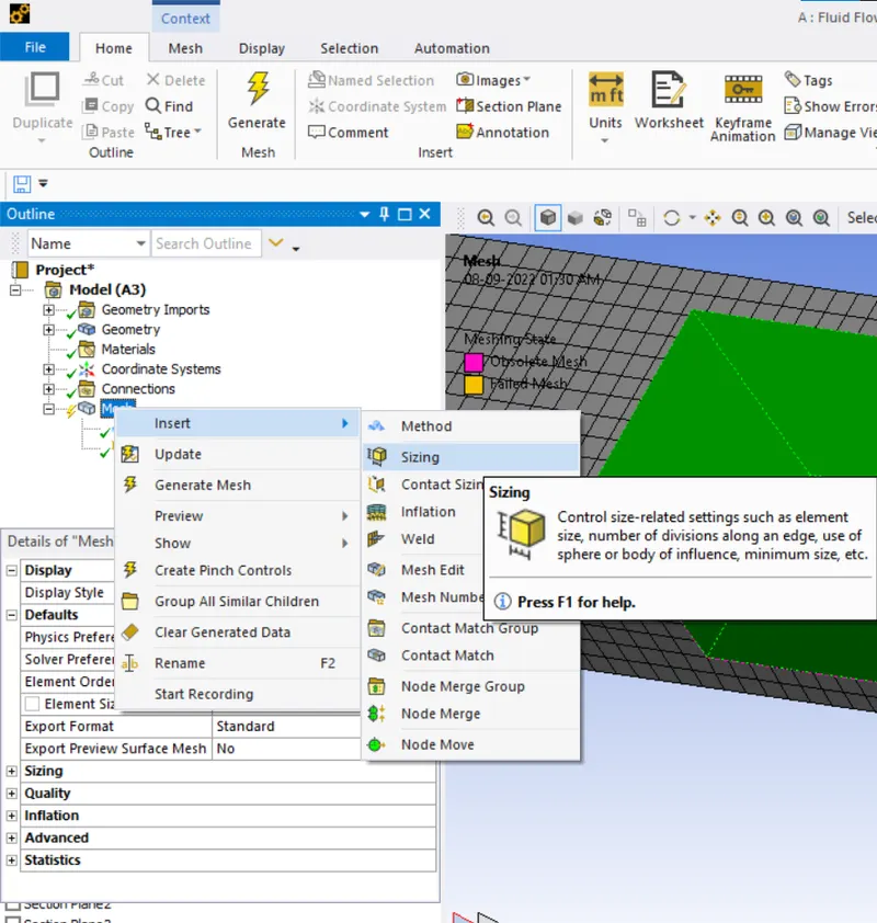
- Selecting the inner enclosure through body selection:
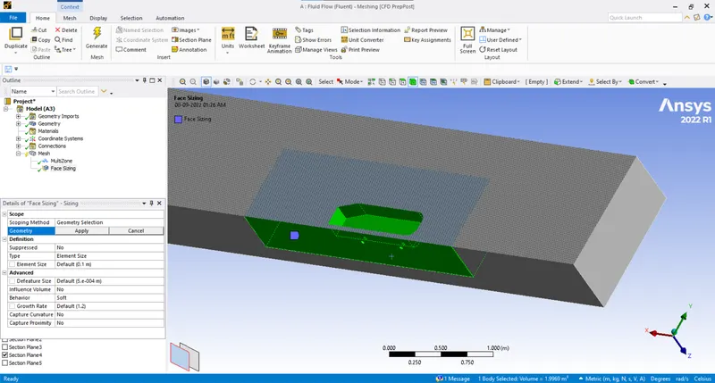
- Defining the element size as 50mm and generating the mesh:
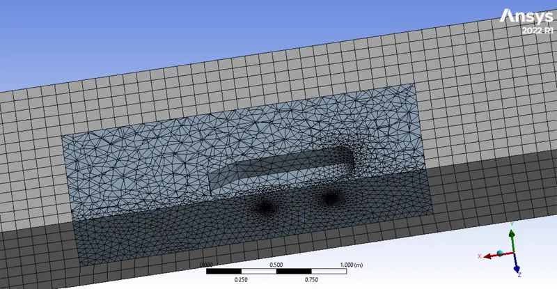
- Now refining the mesh of the faces of the Ahmed Body:
- First hiding the faces not required in this process:
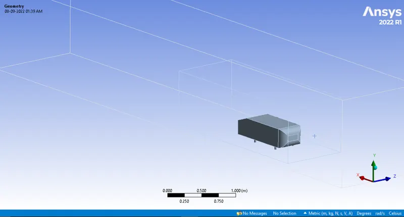
- Select the face and hide it by using the options or use F8.
- Now select the sizing and faces for it:
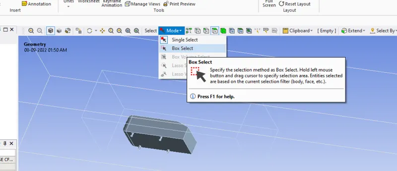
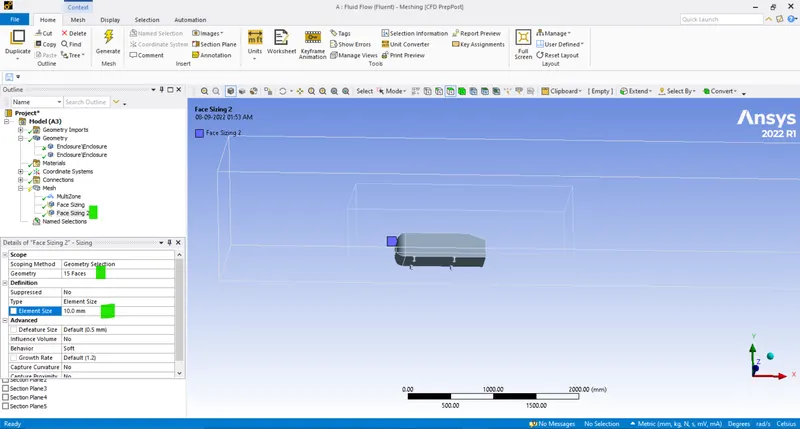
- Also changing the growth rate to 1.1 from 1.2.
- After generating the mesh:
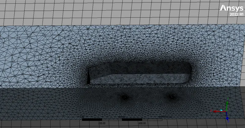
- Now generating the Inflation layers so that the near wall boundary conditions are clearly captures:
- Since the boundary conditions are applied at all the boundaries, so we need to have the centres of the cells which are in contact with the boundary wall of the Ahmed body to be allinged and closley follow the shape of it's outter wall so the boundary conditions are applied accureatly to compute the problem:
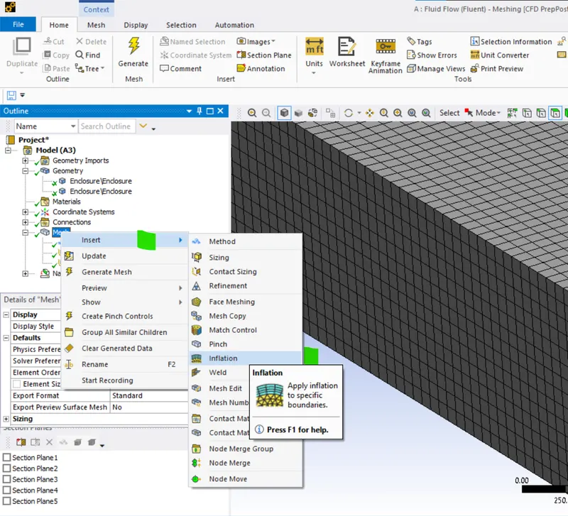
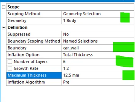
- Here the total thickness is defined by calculating the initial layer thickness and finding it with growth rate, in this case with 6 layers and initial layer thickness of 5 mm we have 12.44mm as total thickness:
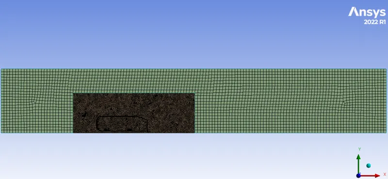
- After meh generation:
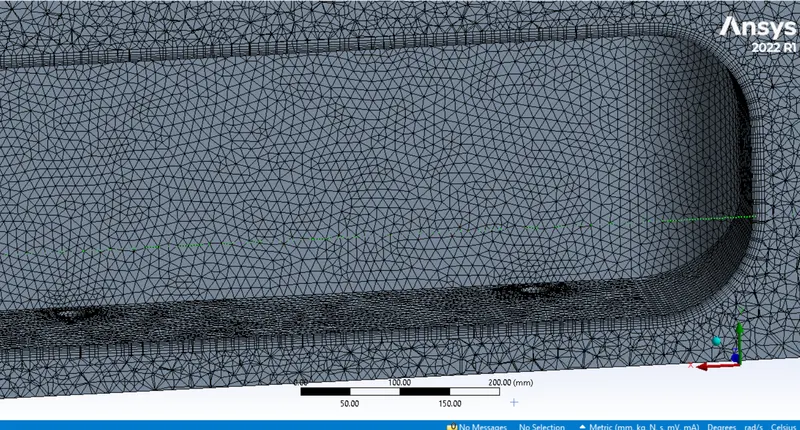
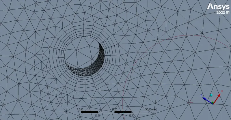
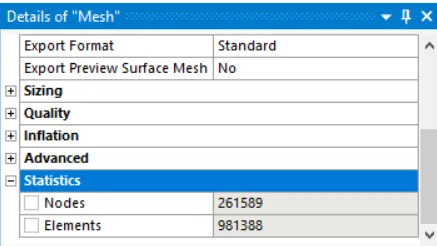
- Total statistics at this point:

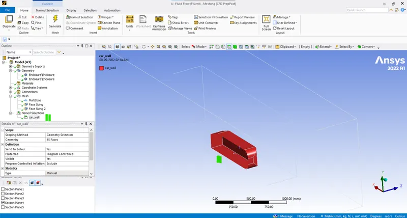
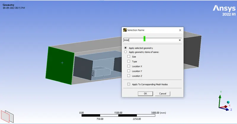
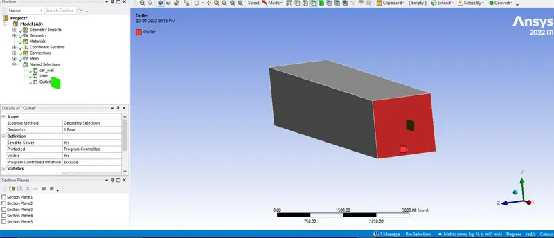
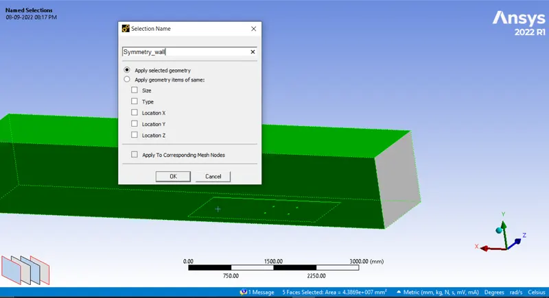
- Naming the components of the geometry:
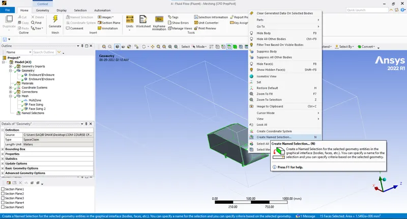
- Ahmed Body walls - car_walls (Select the faces/bodies > N > Define the names):
- Inlet:
- Outlet:
- Symmerty_wall:
- Ahmed Body walls - car_walls (Select the faces/bodies > N > Define the names):
- After naming and meshing the total volume of the geometry is as follows:
- Now setting up the pre-processor (In setup):
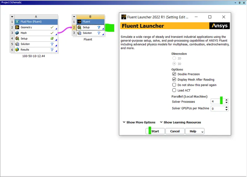
- Open the setup with 4 processors:
- Now as the velocity is 25m/s which is 1/14 Mach number so here we need to use the pressure based solver as the Mach number is less than 0.3.
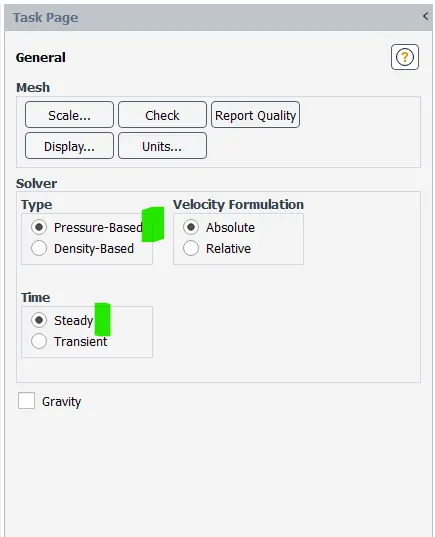
- Here the steady state solver is considered as we do not have to deal with any time dependent output parameter such as Strohaul number.
- Here the Energy Equations are turned on:

- Defining the fluid properties, here we are using the properties of air at 15 degree celsius:
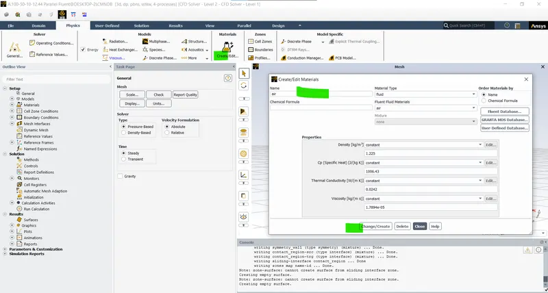
- Definig the properties to the cell zones (Cell zones > select the zone > define the fluid):
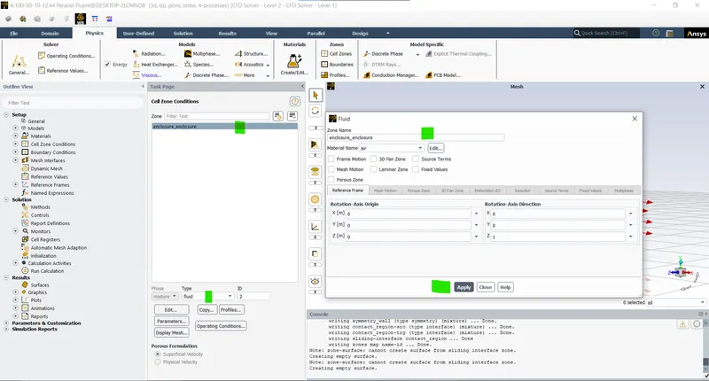
- Defining the boundary conditions:
- Inlet (velocity inlet = 25 m/s):
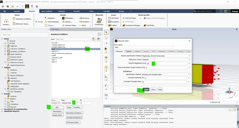
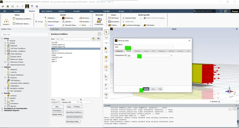
- Outlet (pressure outlet):
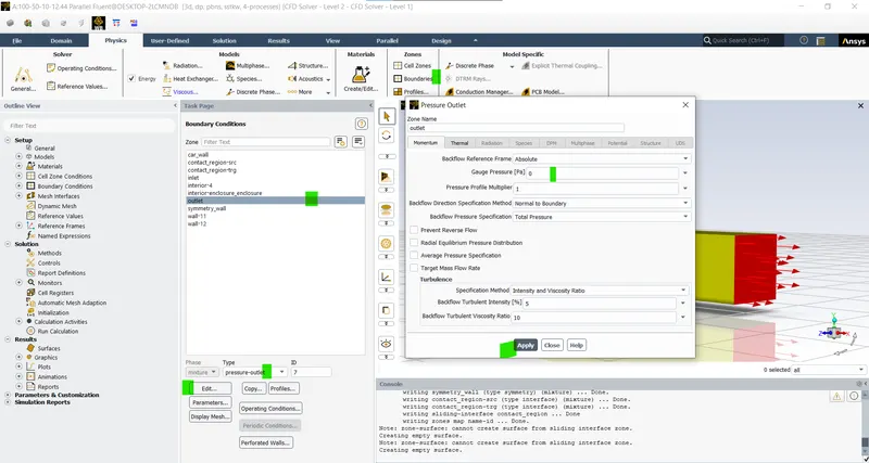
- We are using the as k-omega as the viscous model the flow model as the flow is turbulent and we conserned towards the flow near the boundaries which is best done by the k-omega model (Re = 658184):
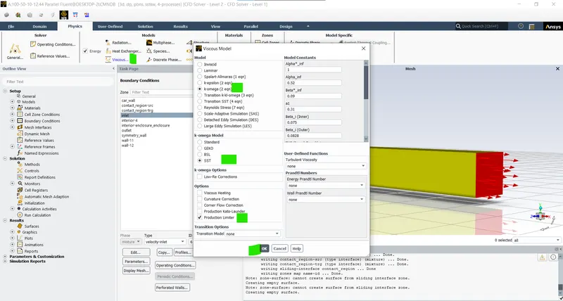
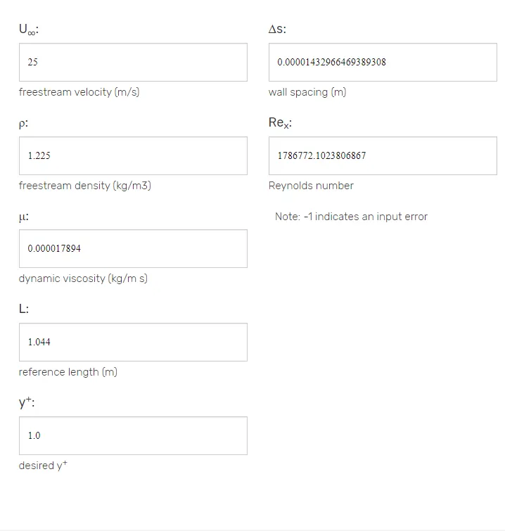
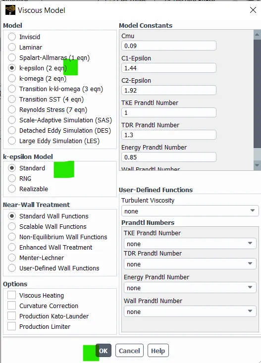
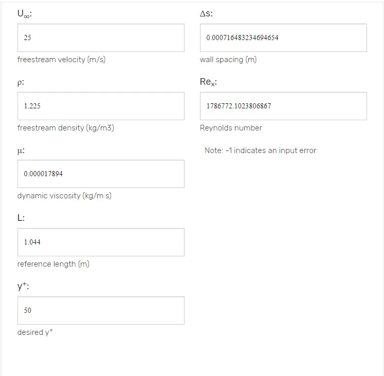
- Here as can observe that if we need to use k-omega model we need to have y+ value as 1 which will lead to initial first layer thickness of 0.01mm which will intern cause more element and computation power so sor this study we are taking the k-epsilon model which has first layer thickness of 0.7mm for y+ of 50.
- Creating the plane visualize the velocity pressure contours:
- Here the plane is along xy plane and has normal along z plane.
- The plane generation method selected is point and normal(at z) (Results > create plane > point and normal > xyz at 0 and normal at z > create):
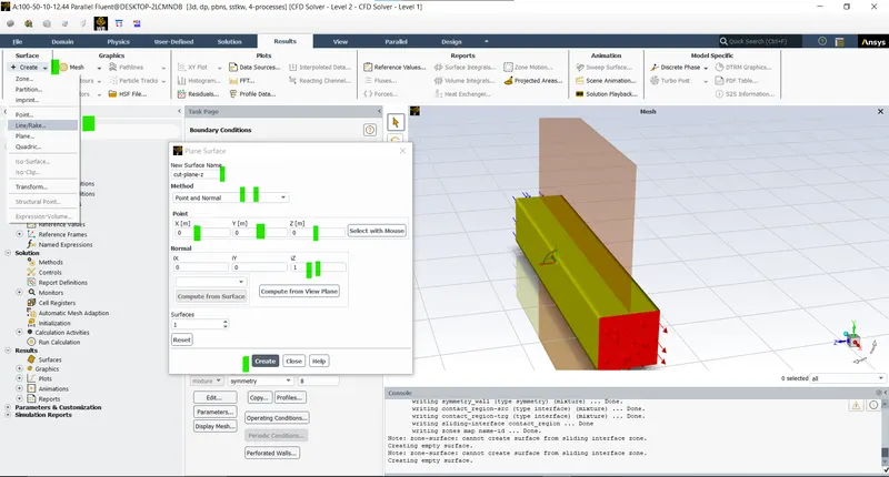
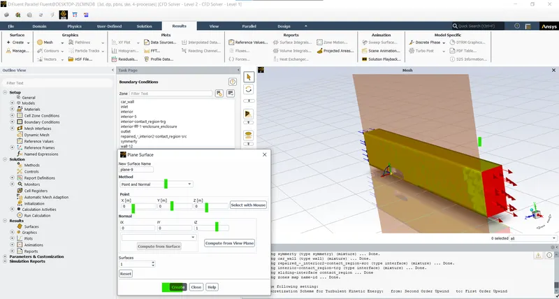
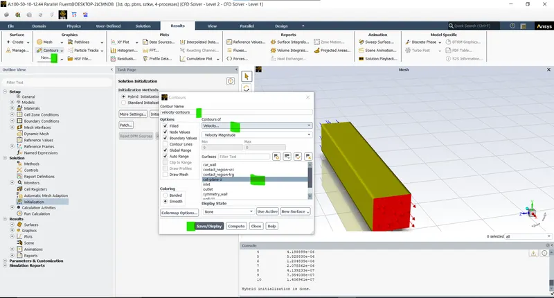
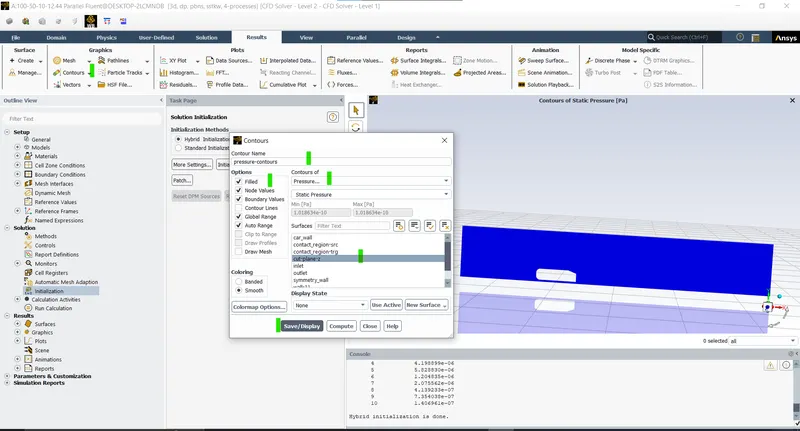
- Creating the contours for velocity and pressure contours (Results > Contours > New > Select the parameter and plane > Ok):
- Velocity contours:
- Pressure contours:
- Creating the animation of the contours through the iterations (Solutions > Activities > Create > Solution animation > select the view > select the parameter contour > Ok):
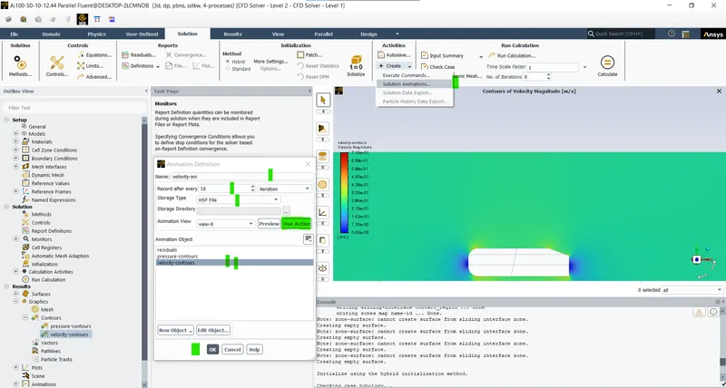
- Definition for the parmaters:
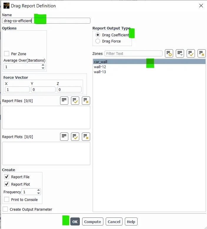
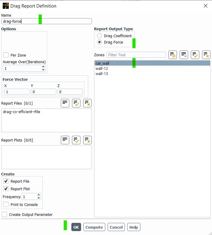
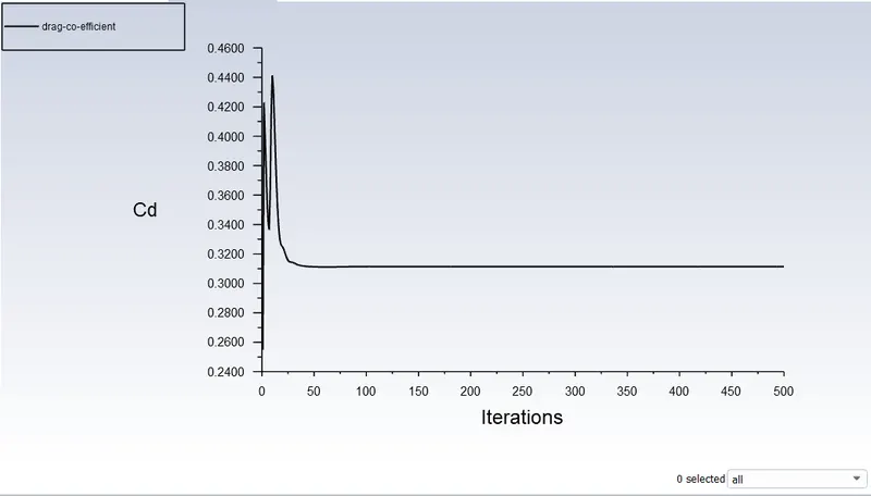
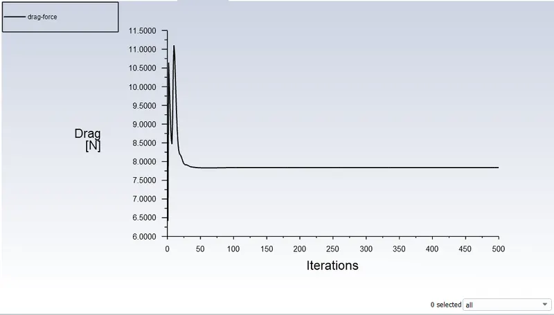
- Drag force and drag co-efficient:
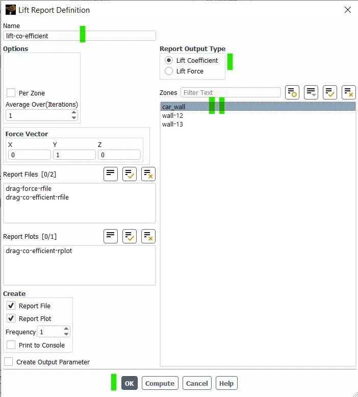
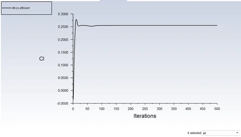
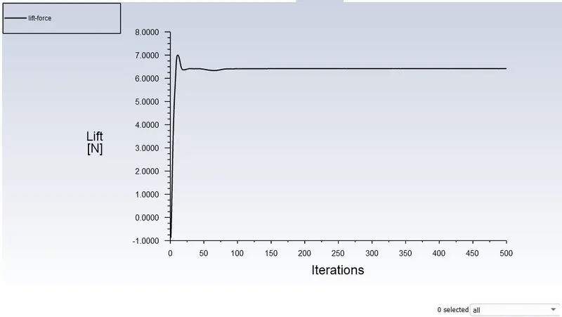
- Lift force and lift co-efficient:
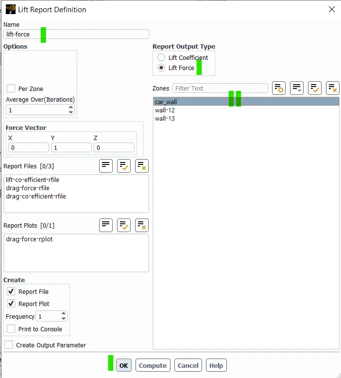
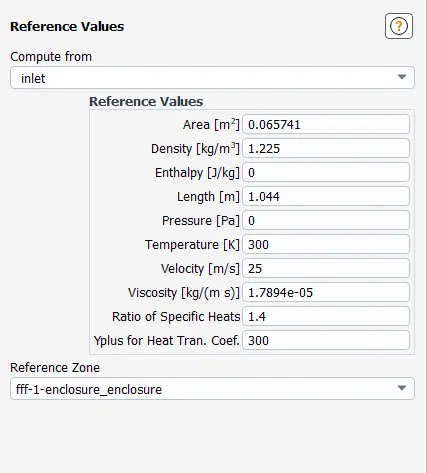
- Now definig the reference values:
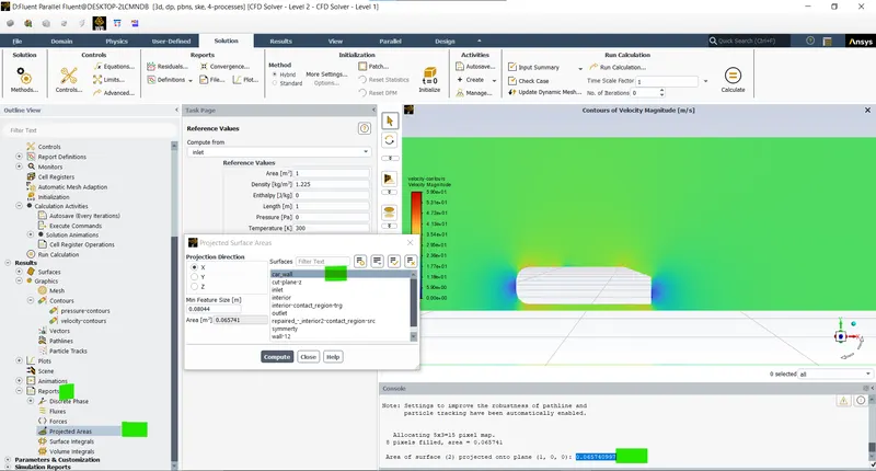
- Here we need to find the frontal area as Results > projected areas > select the car_wall > In x-direction:
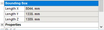
- Here the area is 0.065740997 sq.m and the length is 1044mm.

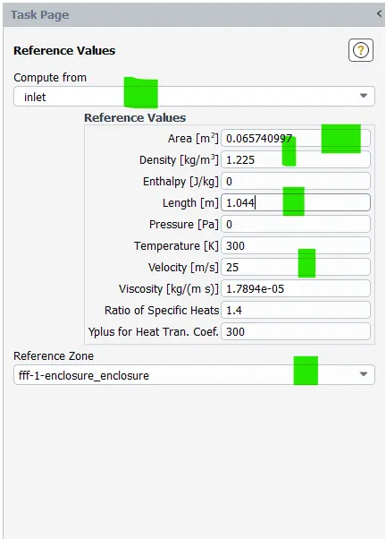
- Now as the pre-processing is complete we can now move the processing or solving.
- Open the setup with 4 processors:
- Processing:
- Here we are using the Hybrid Initialization as it sutable for steady state solver as it solve the potential flow eqautions with stream function and velocity potential, we need to worry about the assumption made as the initial conditions will be washed away as the iteration progress:
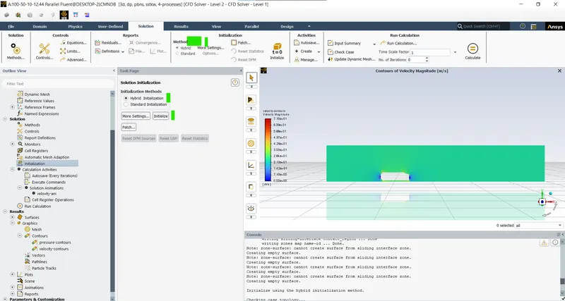
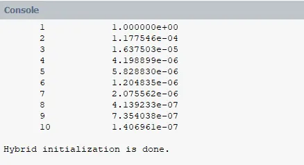
- As we can see the solution is converged we can proceeed to the running the solver setup:
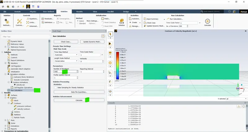
- Here the solution is run for 500 iterations:
- Post-processing:
- Here the results obtaines are extracted and analysed with more flexibility.
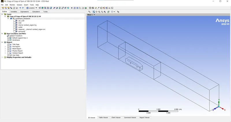
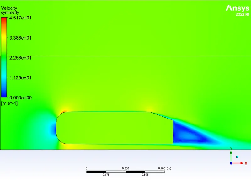
- Now as we need to analyse the wake region we are going add planes to view contours for the parts:
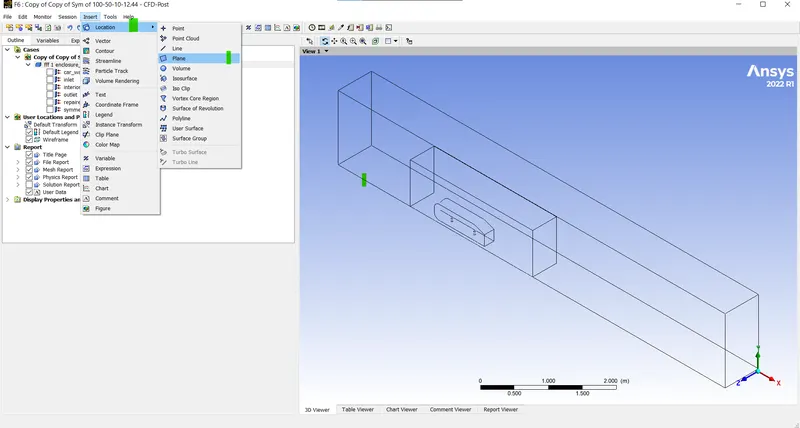
- Adding the plane:
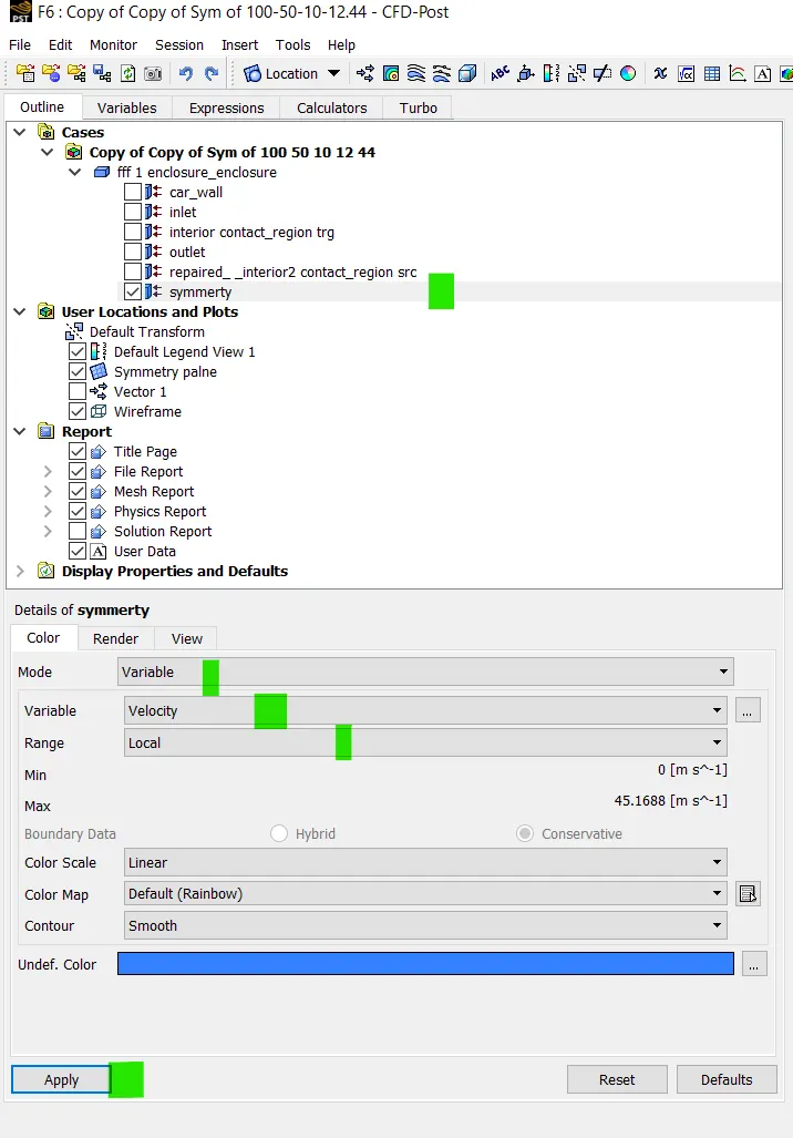
- Velocity contours (mode > variable > velocity > ok):
- Pressure contours:
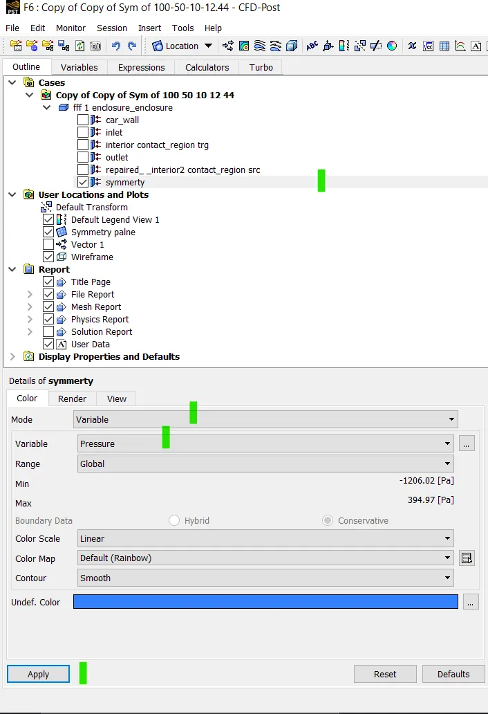
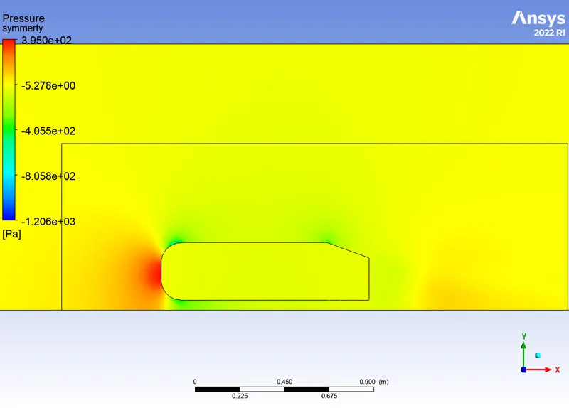
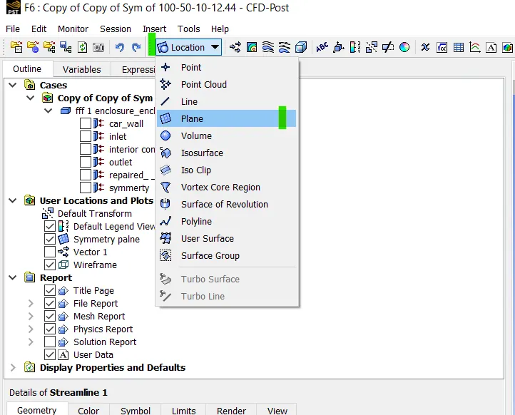
- Inserting planes in yz plane to visualize the wake region (Location > Plane > yz plane > distance > ok):
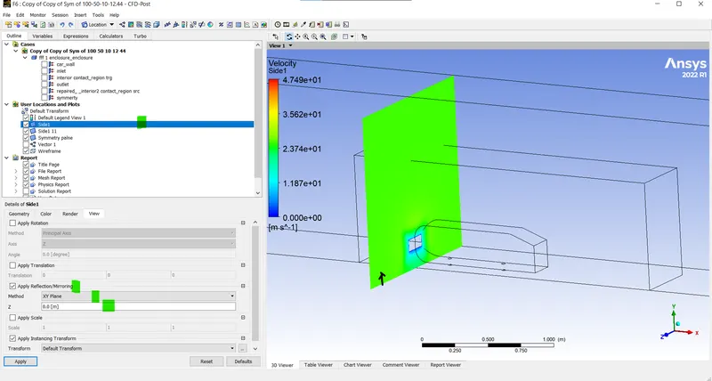
- Now mirroring the plane for symmetric view:
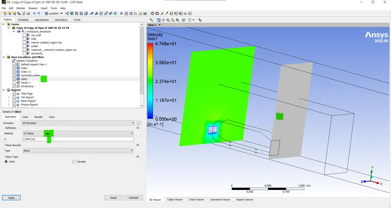
- Seconde side plane:
- Mirror (duplicate the plane and mirror it):
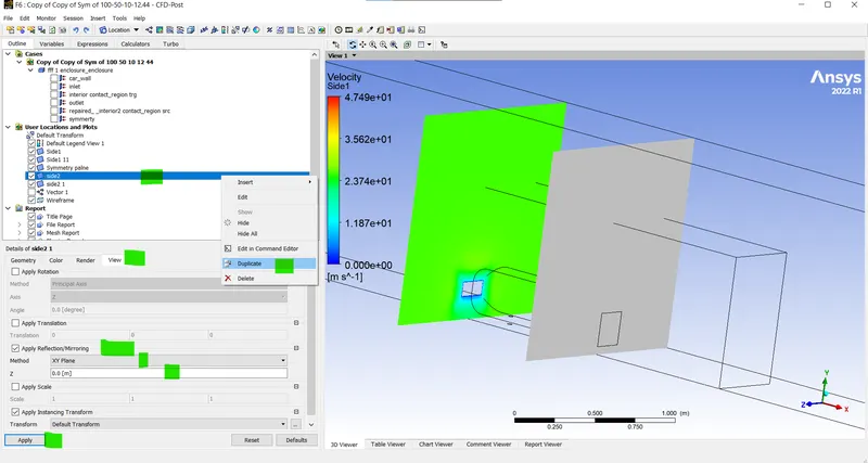
- Now all the plane are total of 5:
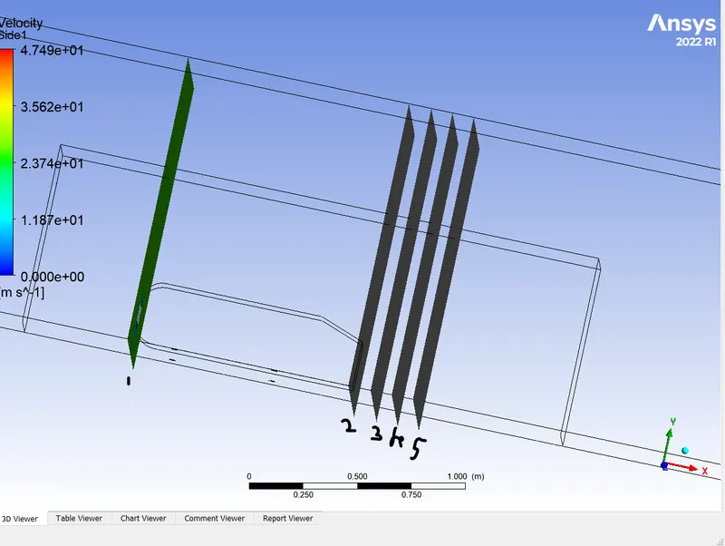
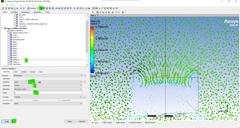
- Vector (Vector > select the palne > variable > ok):
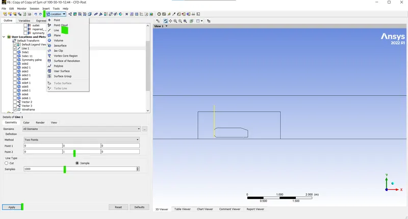
- Inserting the line for plotting the velocity plot:
- Create a line (Location > line > co-ordinates > ok):
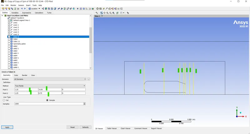
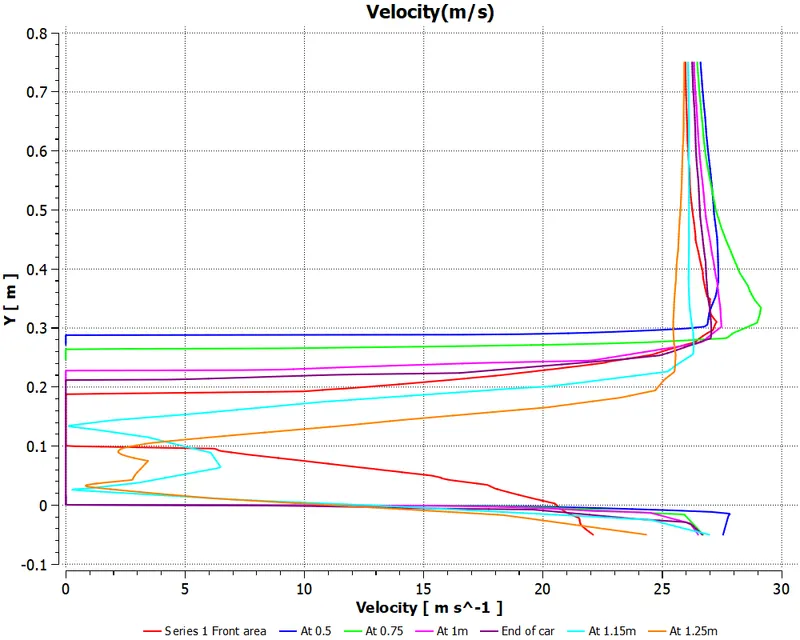
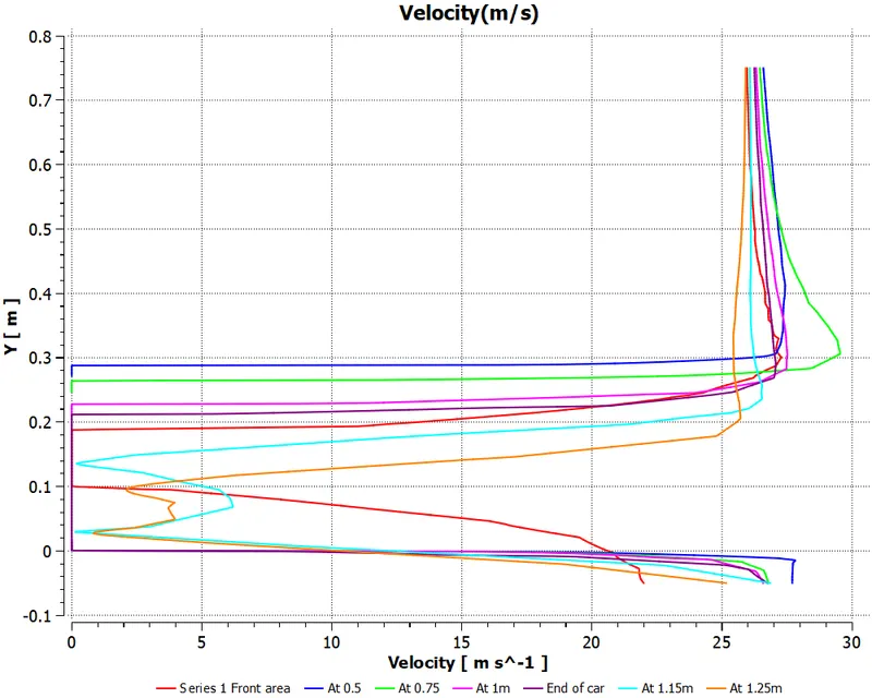
- Plotting the y distance vs velocity graph (Insert chart > select the series > define x and y axies > apply):
- Here x-axis is the velocity(m/s) and y-axis is the distance in y direction:
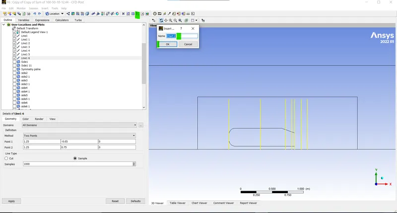
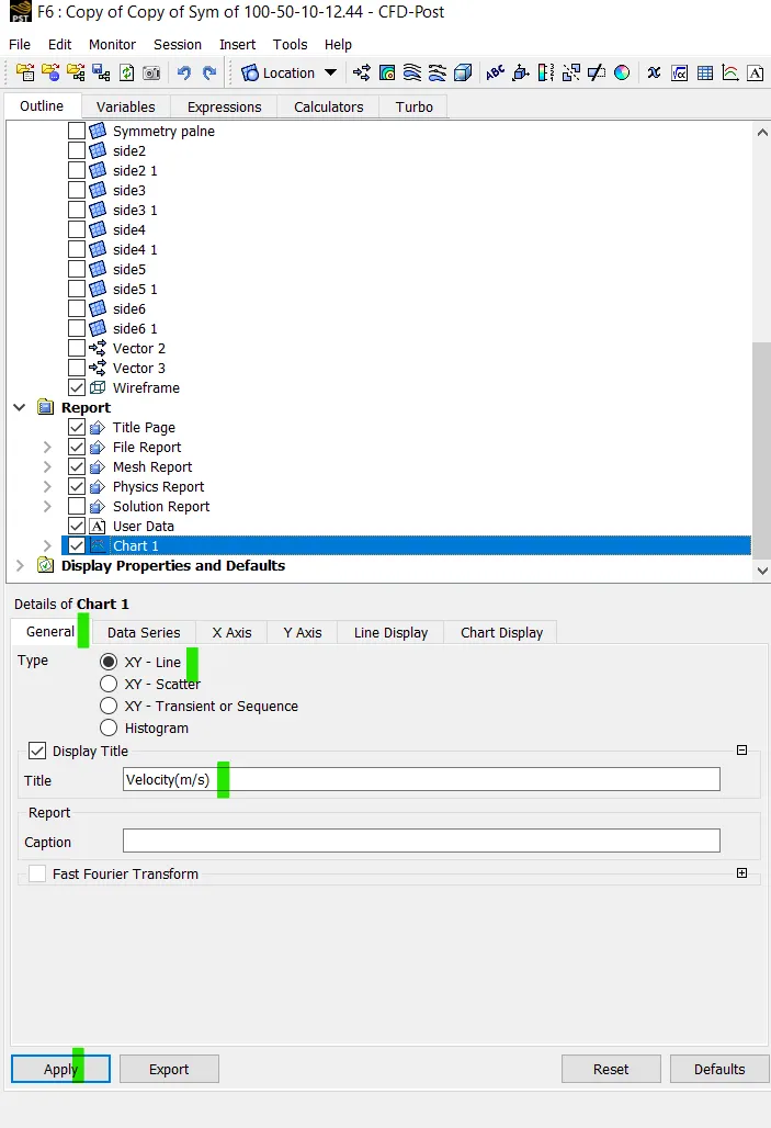
- Add the series at the lines:
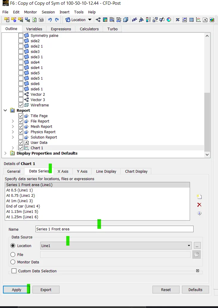
- Defining the x-axis:
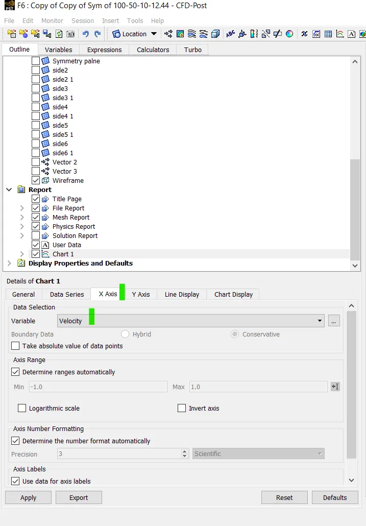
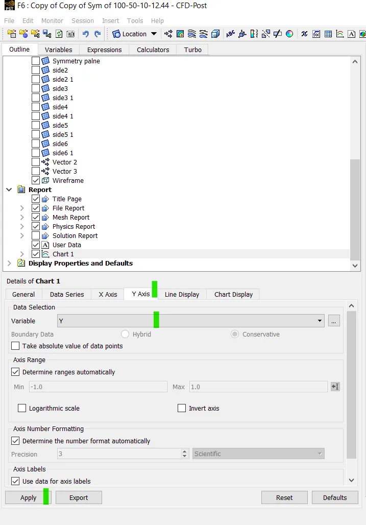
- Defining the y-axis:
- Plotted graph:
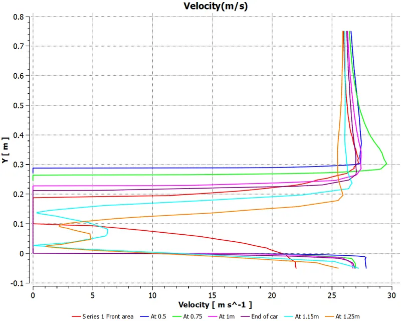
- The graph shows the variation of velocity through y direction at different lines to represent the flow velocities and specially the flow seperation and wake region behind the car model.
- The flow near the car walls are showing the zero sslip condition.
- At the end of the car we can see the wake region caused, the wake region seperates the fluid flow over the body so it creates negative pressure graident and reverses the flow as seen in the graph (at 1.15 and 1.25m).
- At the end of the car there is vaccum/low pressure region which has much influence on the drag as the fluid around the region can't imediatly fill the region.
- Grid Independency test:
- There are three cases considered for the grid independency test:
- First with 100mm for outer enclosure, 50mm inner enclosure and inflation of 0.7 mm with 1.2 growth rate:
- Now the total mesh count is 109953
- Second with 75mm for outer enclosure, 30mm inner enclosure and inflation of 0.7 mm with 1.2 growth rate:
- Now defining the element length to be 75 mm for outer and 40 for inner enclosure:
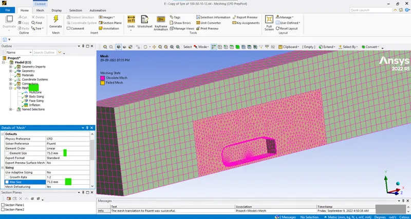
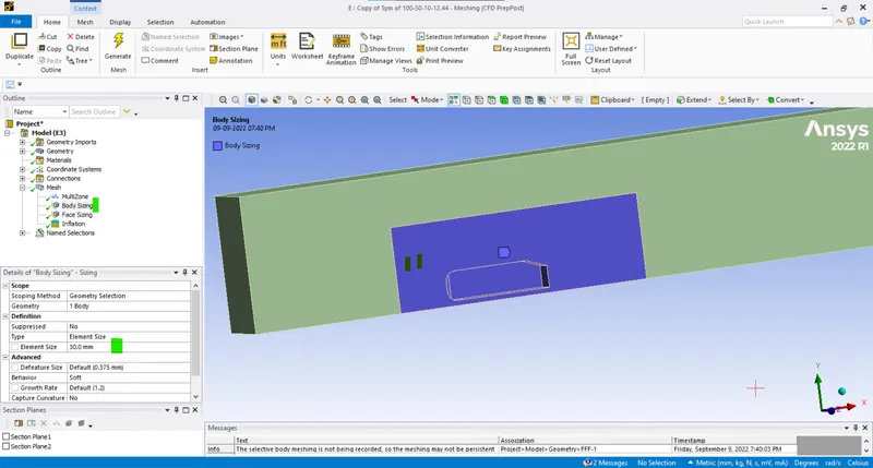
- As we are have only 0.3 million cell count so refining again, inner enclosure to 25mm:
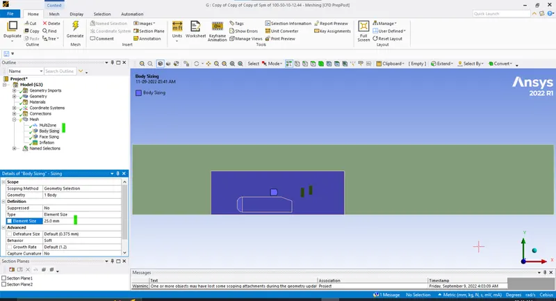
- Now the cell count is more than half a million:

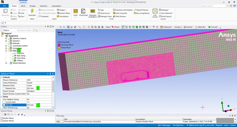
- Third with 60mm for outer enclosure, 20mm inner enclosure and inflation of 0.7 mm with 1.2 growth rate:
- Refining the mesh for outer enclosure:
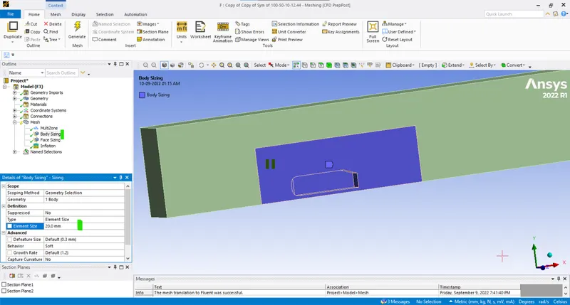
- Refining the mesh for the inner enclosure (20mm):
Results:
- Case-1:
- Mesh count:
- Outer enclosure = 80mm.
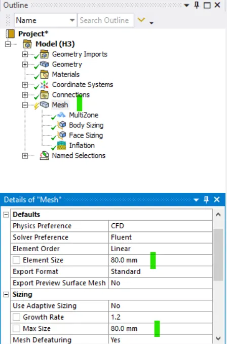
- Inner enclosure = 30mm:

- There are totally 346810.
- Reference values:
- Residuals:
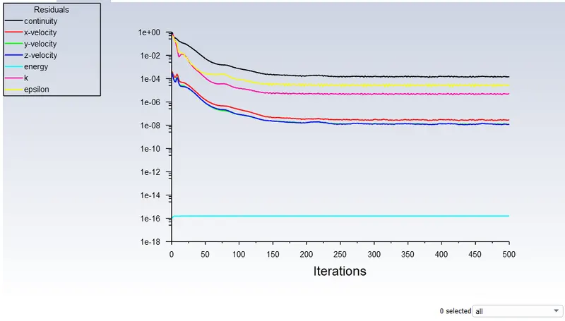
- The results are converged at 91 iterations but for the flow visuatization solver is run for 500 iterations.
- Drag co-efficient and drag force:
- Lift co-efficient and lift force:
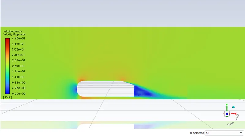
- Velcoity contours:
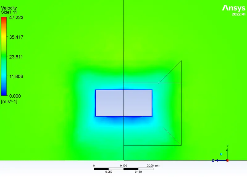
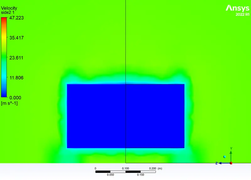
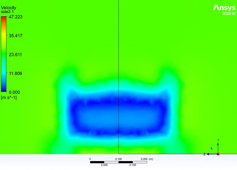
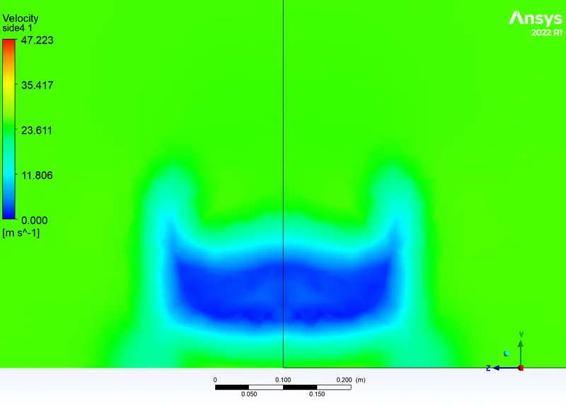
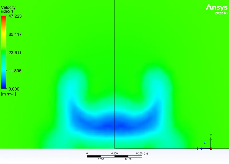
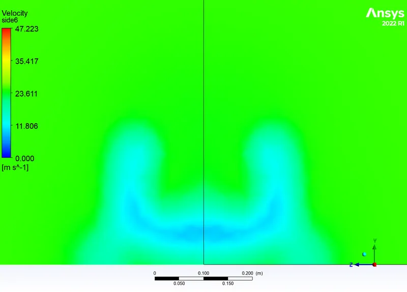
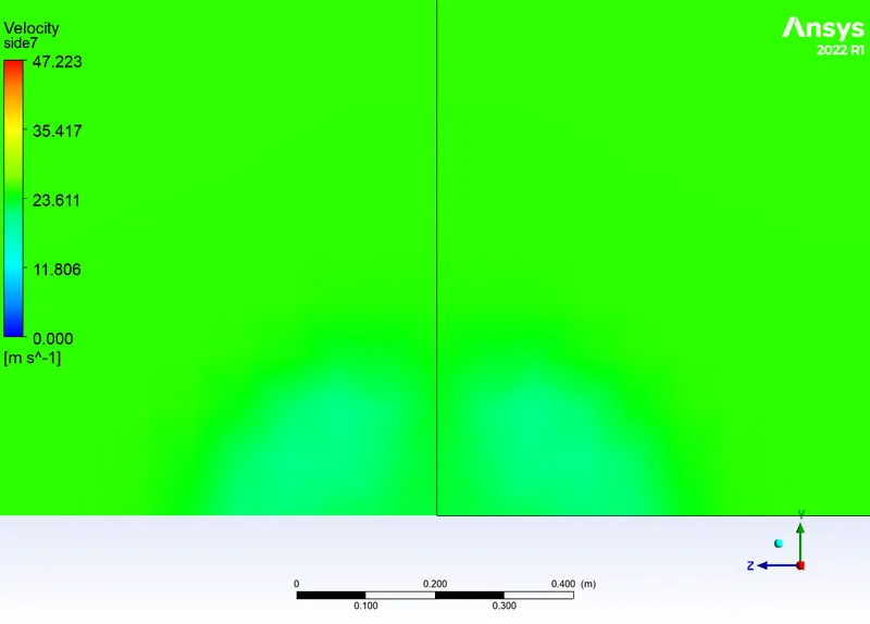
- Above contour at 2.3 m from front of car.
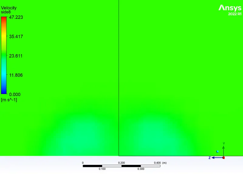
- Above contour at 2.8m from the front of the car frontal area.
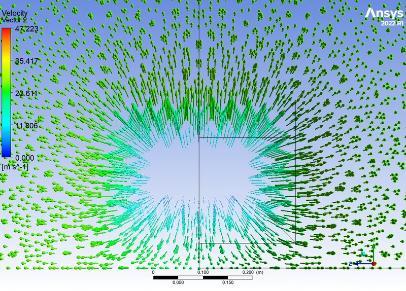
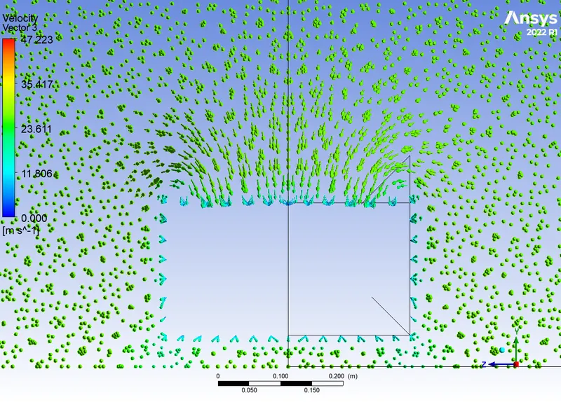
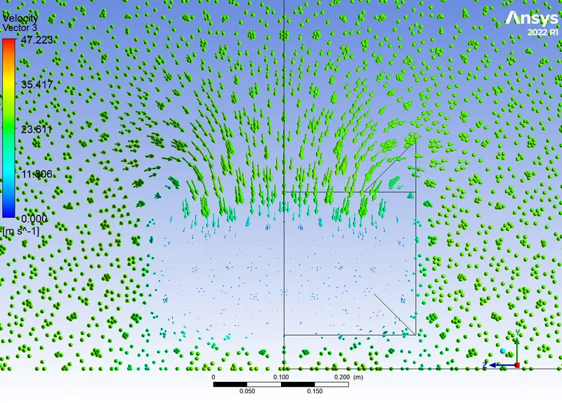
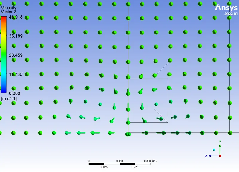
- Velocity vectors:
- Stream lines (velocity):
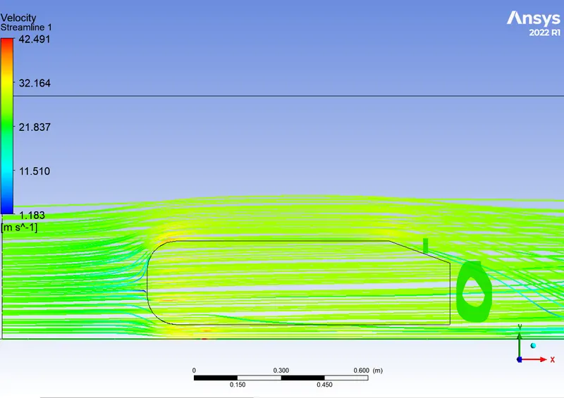
- Here we can clearly see the wake region, point of seperation and low pressure/vaccum region as marked in the above stream line figure.
- Pressure contours:
- Graph:
- Mesh count:
- Case-2:
- Mesh count:
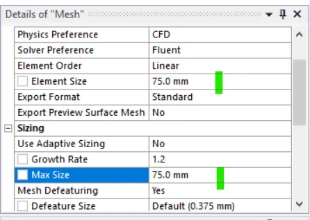
- There are 562785 cells.
- Velcoity contours:
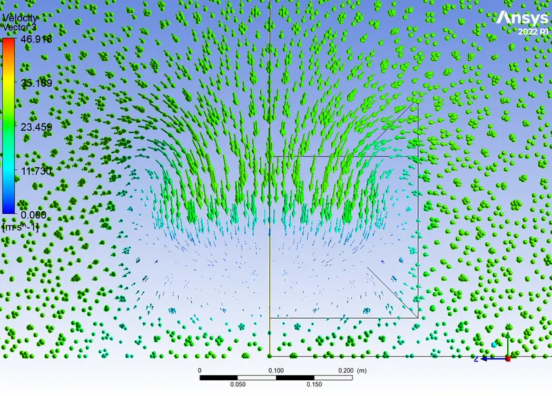
- Velocity vectors:
- Pressure contours:
- Graph:
- Mesh count:
- Case-3:
- Mesh counts:
- Velocity contours:
- Pressure contours:
- Velocity contours:
- At Plane1:
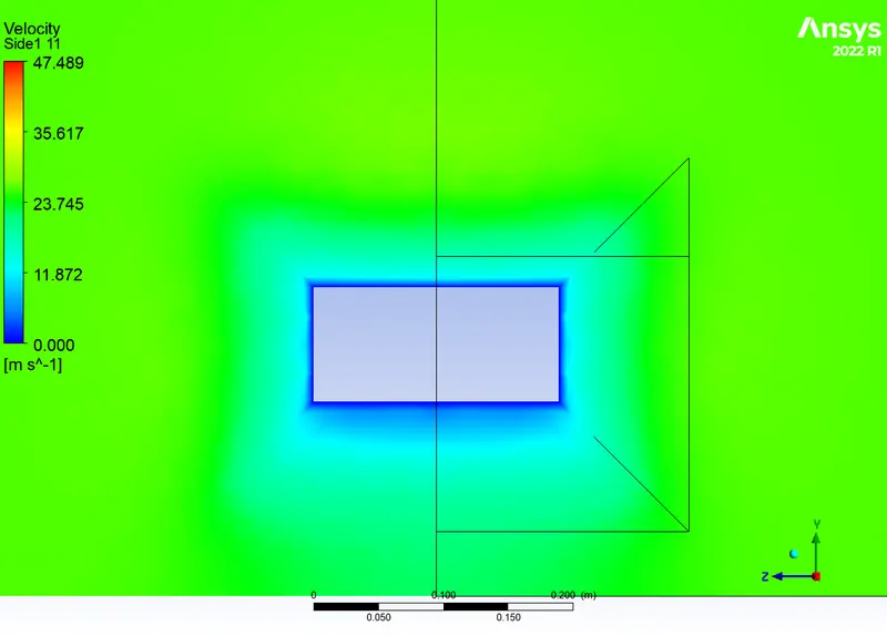
- At Plane2:
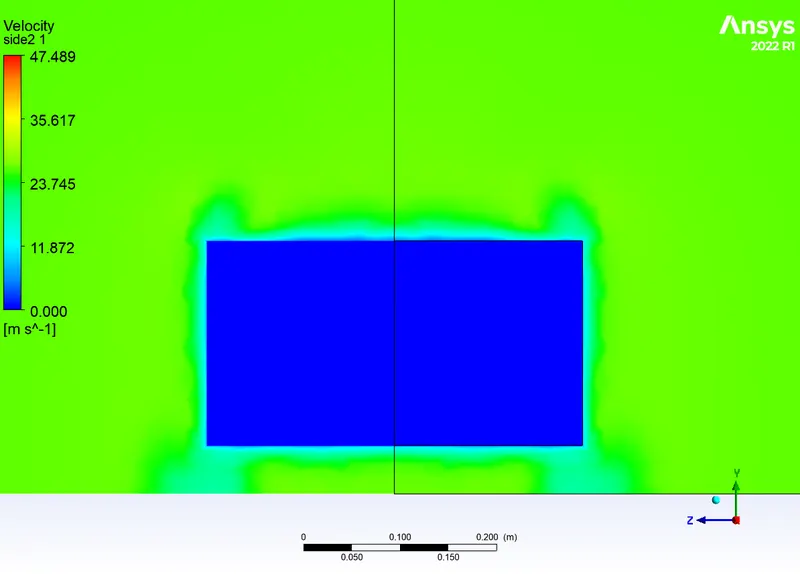
- At Plane3:
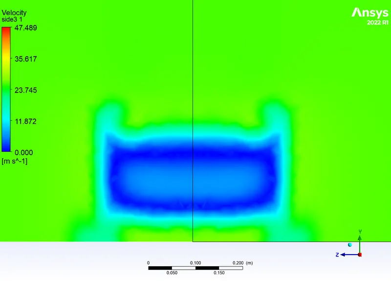
- At Plane4:
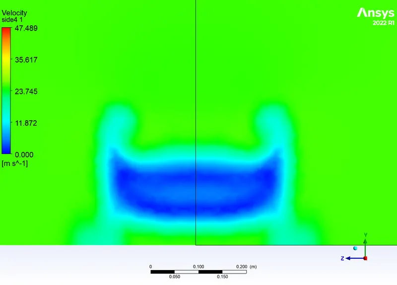
- At Plane5:
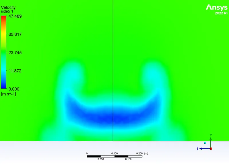
- At Plane6:
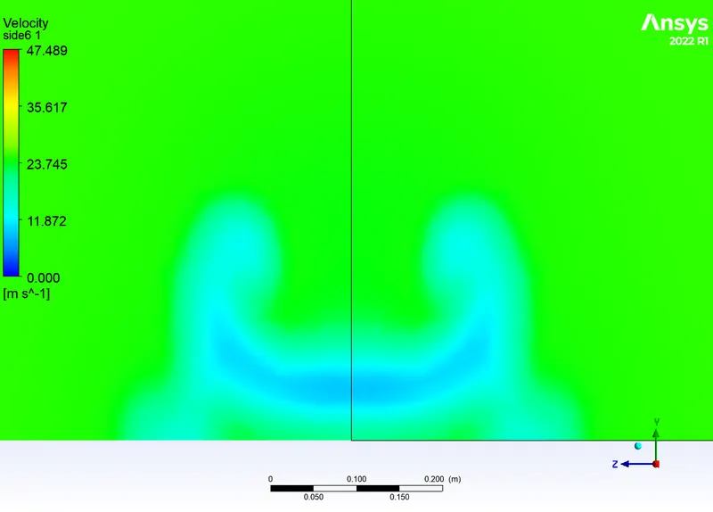
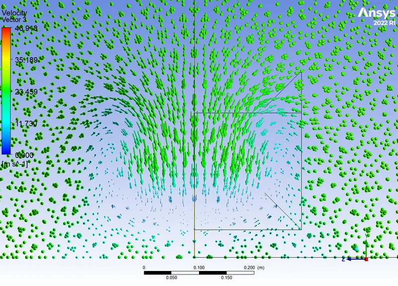
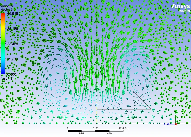
- Velocity vector:
- At Plane2:
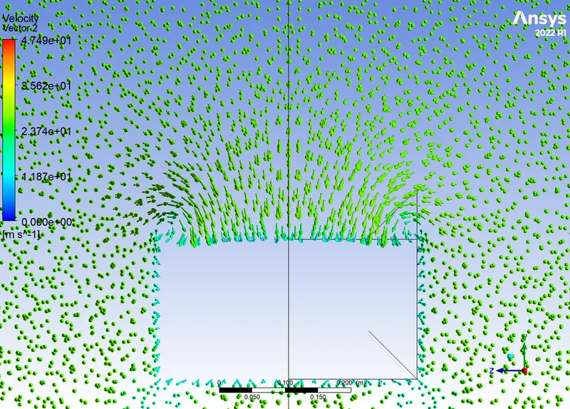
- At Plane3:
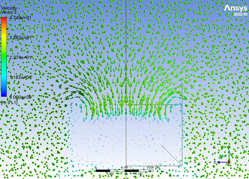
- At Plane4:
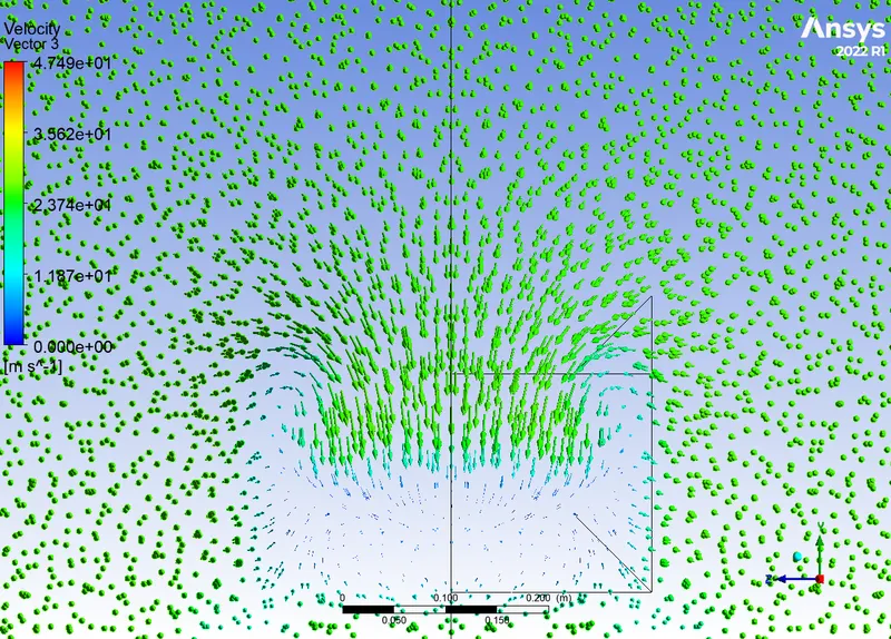
- At Plane5(1.35m):
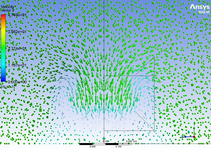
- At Plane6 (1.45m):
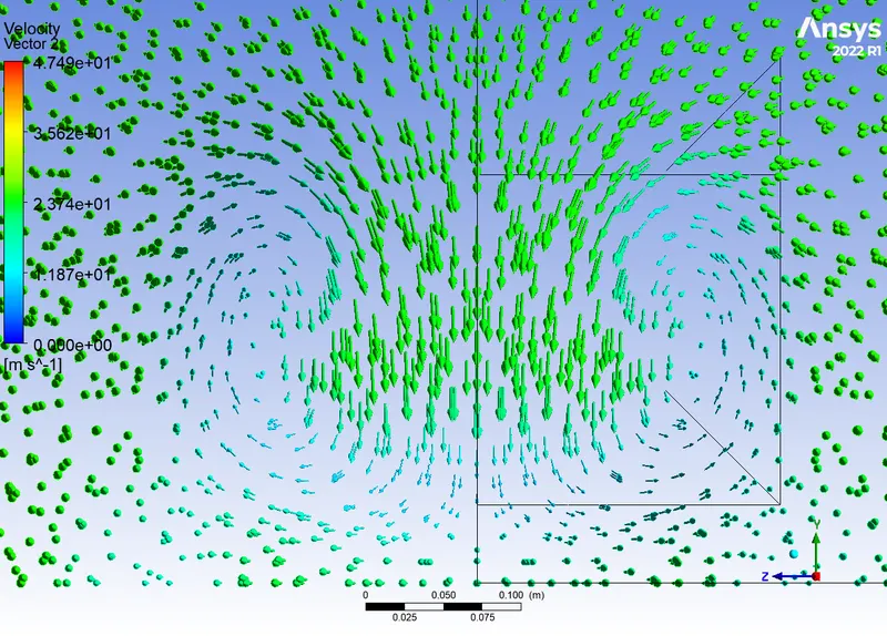
- Pressure contours:
- Velocity chart:
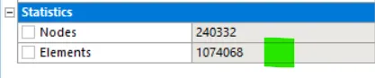
- Mesh counts:
- Results table:
-
Sl.no Outer/inner No. of Elements Drag co-efficient (Cd) Lift co-efficient (Cl) Drag Force Lift Force 1 80/30mm 346810 0.31140619 0.25511412 7.8369960 6.4203229 2 75/25mm 562785 0.30219649 0.26132941 7.6052203 6.5767401 3 60/20mm 1074068 0.29266851 0.25160958 7.3654348 6.3321262
-
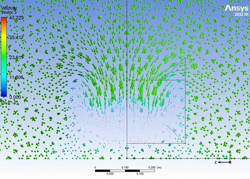
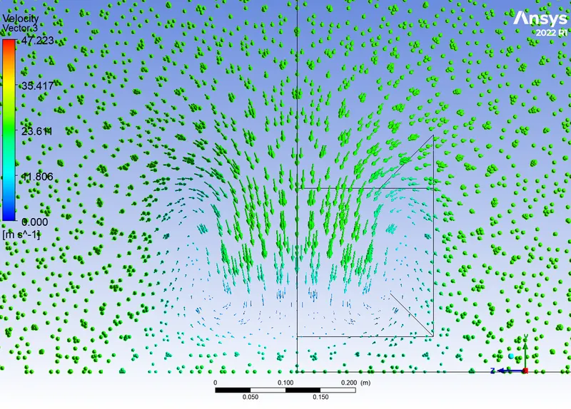
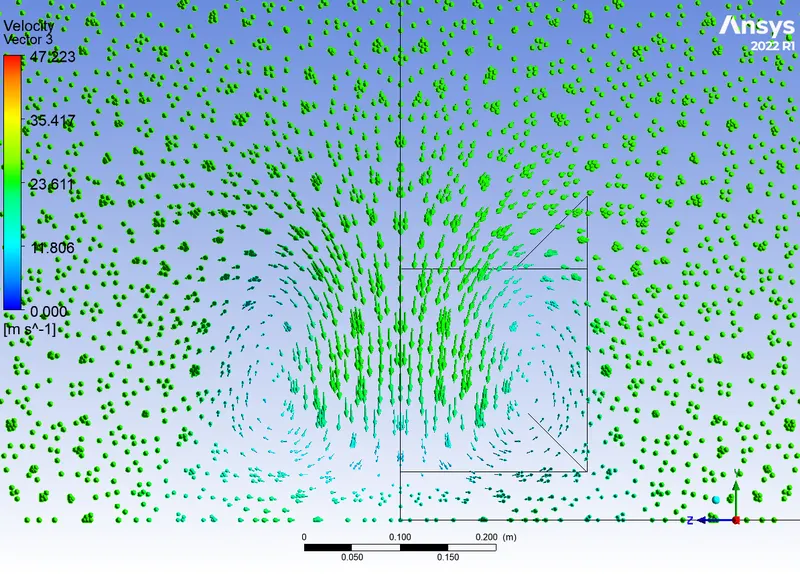
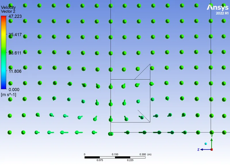
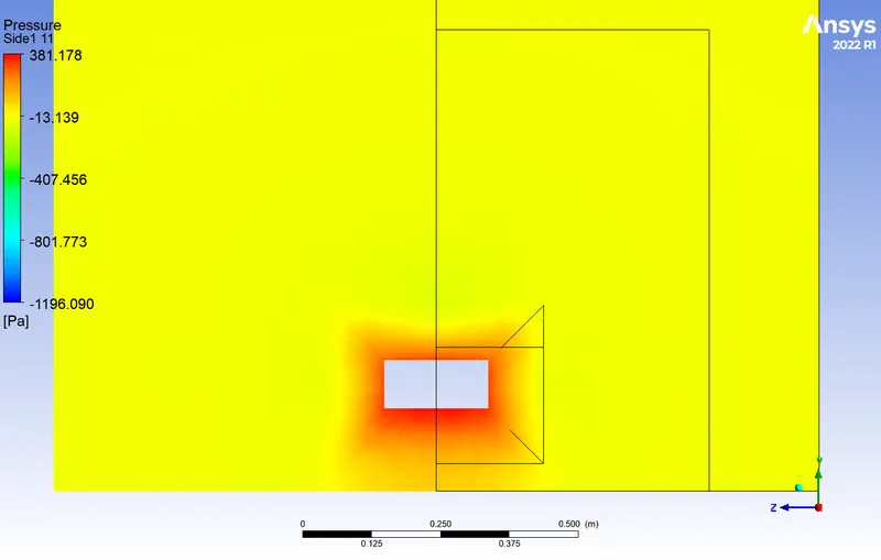
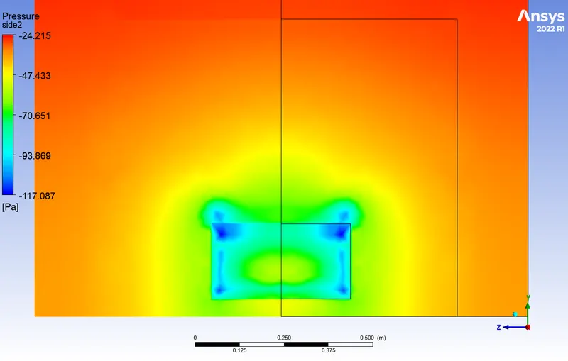
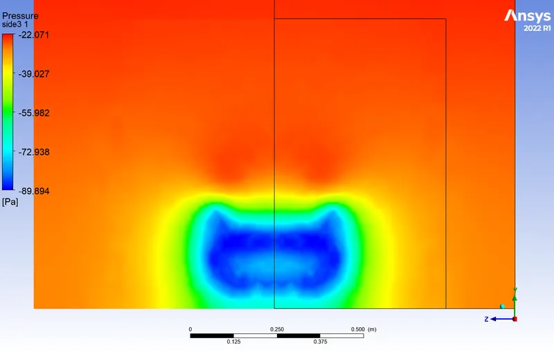
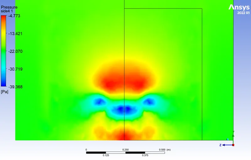
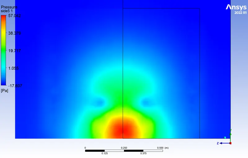
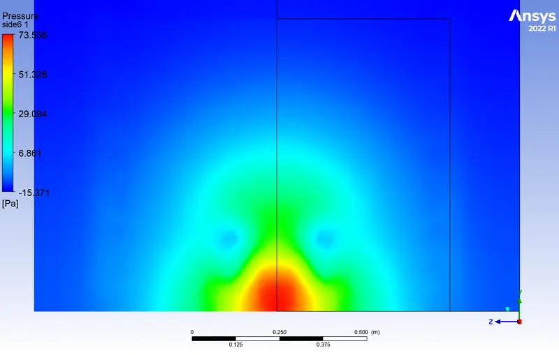
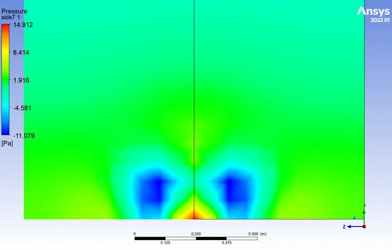
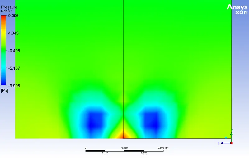
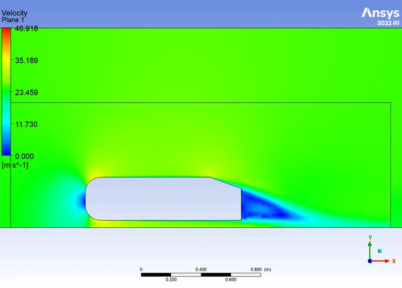
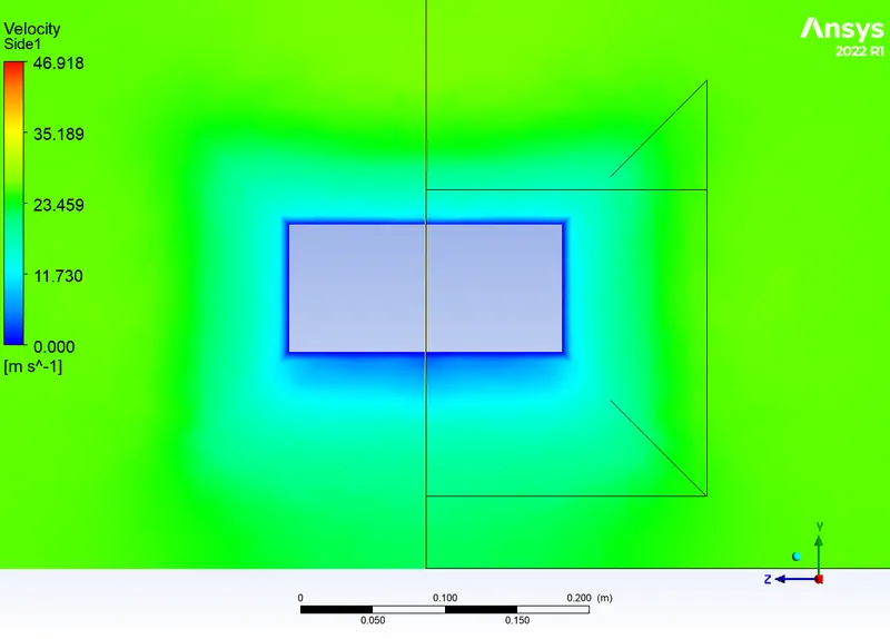
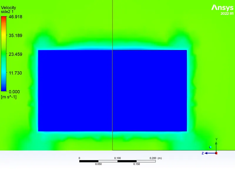
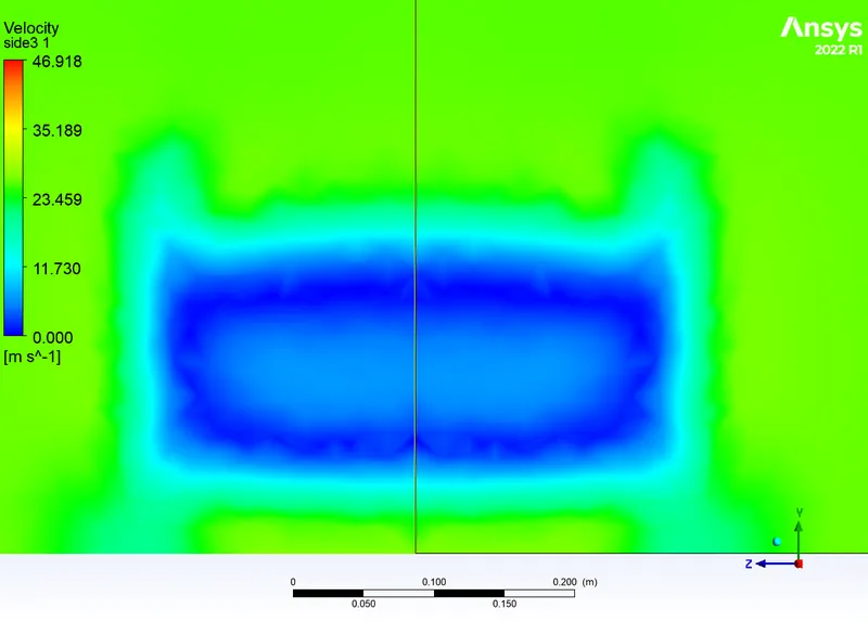
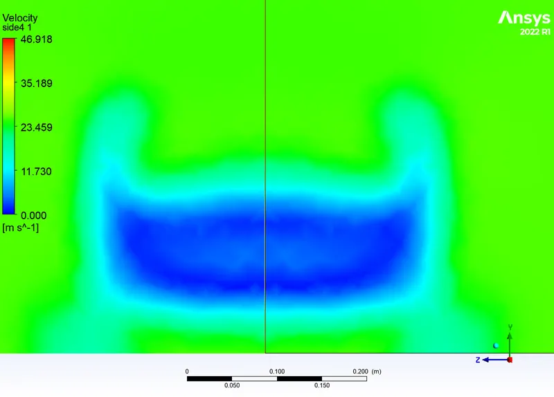
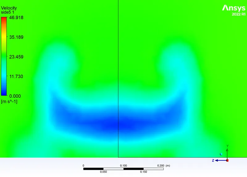
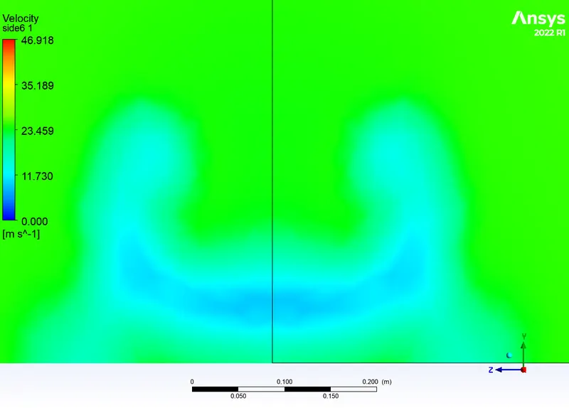
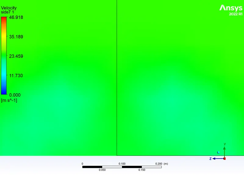
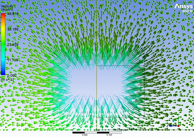
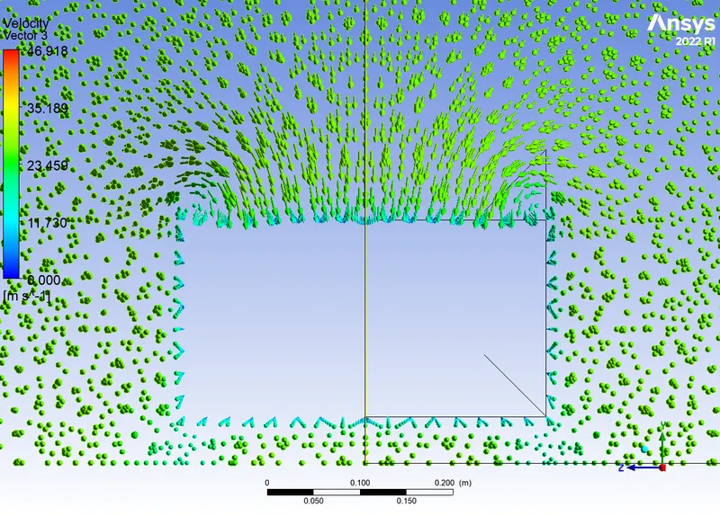
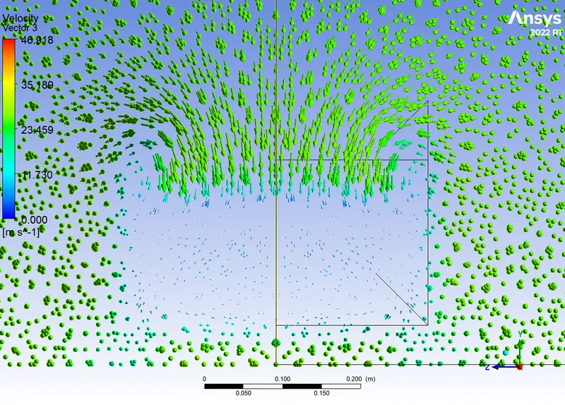
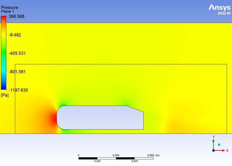
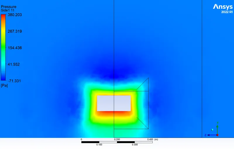
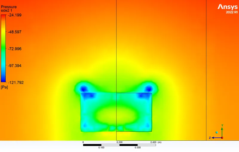
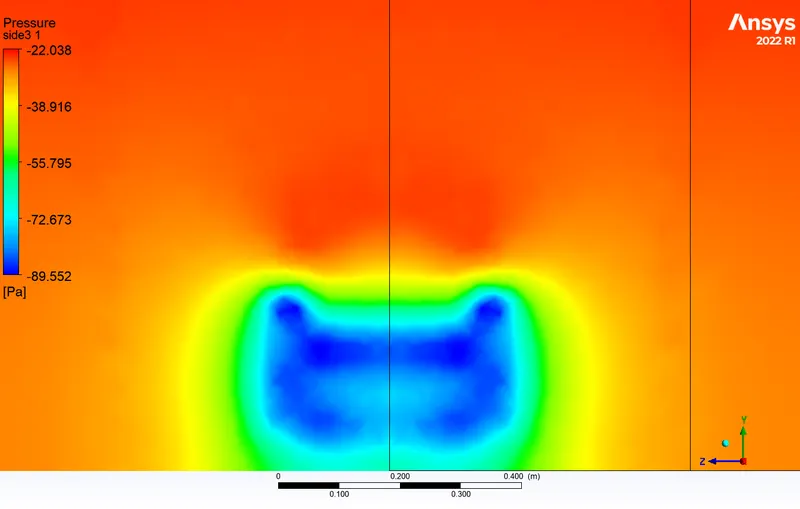
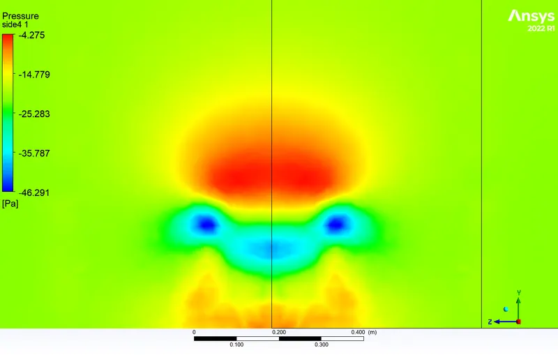
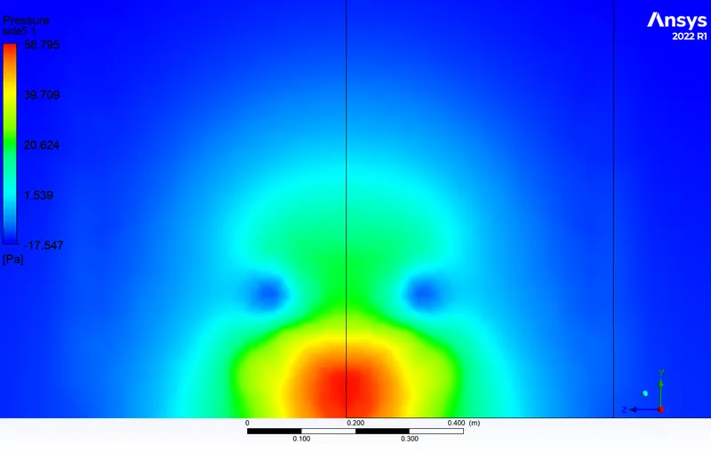
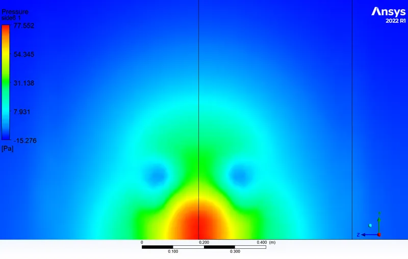
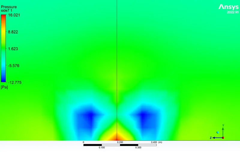
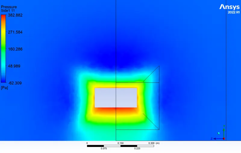
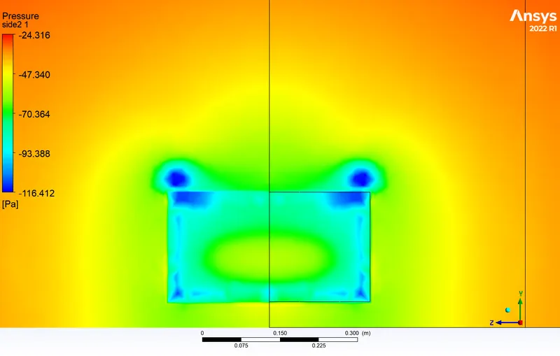
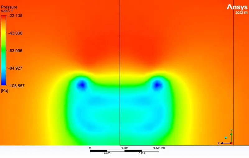
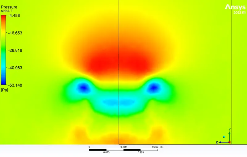
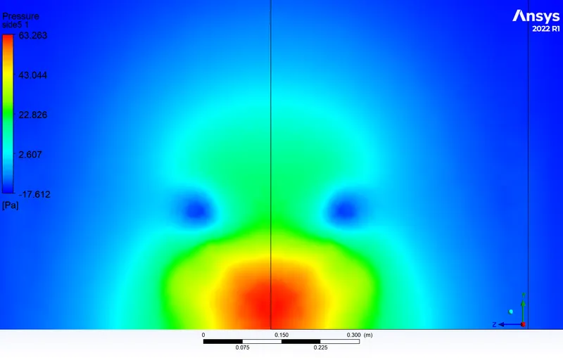
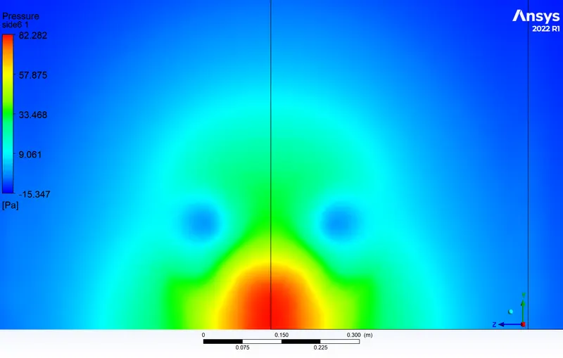
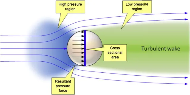
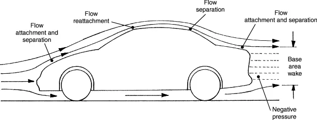
As the car is moving relative to the fluid it pushes all the fluid in it's path away and as the vehicle moves it creates an empty low/pressure region behind the car as the volume left behind the car is not filled by the fluid from the side imediatly so creating an low pressure region.
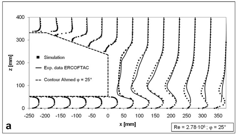
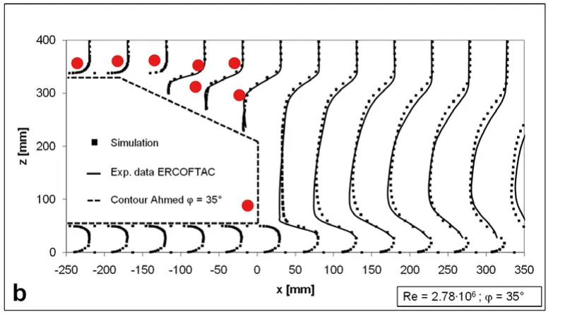
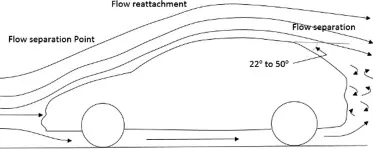
When there is change in the surface curvature the fluid flowing over it detaches from the surface at the point/line of seperation causing the wake region behind which has very low pressure.
Questions:
Q1. Describe Ahmed's body and its importance.
Ans:
- Ahmed's Body represents the generic model of a automobile which is validated with the most of the automobile models present.
- The experimental data obtained from this body is used as standard to compare and analyse the predicted results of the model.
- It captures the flow features around the automobile body.
- It is helpful in understanding the flow patterns and conditions/consiquences arising with it.
- It can be used as the basic model to run the tests or carry out the study on so that the results comply with most of the automobile bodies.
- It is the baseline for the automobile external body aerodynamic simulation.
- It is most helpfull in understanding the flow patterns and behaviour around the external automotive body.
- It can be taken as standard benchmark for study as it fits most of the automotive body.
Q2. Explain the reason for the negative pressure in the wake region.
Ans:
- Whenever there is change in curvature of the body fluid flow seperates (adverse pressure gradient).
- As the fluid flow is detached there is nothing between the surface and seperated fluid layer which causes a lower density region causing the near vaccum or low pressure or negative pressure region.
- This results in the Lower/negative pressure in the wake.
- In other words when there is flow seperation the pressure above the flow regime is high but as there is nothing or very less amount of fluid particles present below the flow regime and the fluid around the body is not able to immedialty fill this region due to the velocity/inertia forces dominating the flow, so there is near vaccum or low pressure region in the wake region, this causes the vortices to form as negative pressure will try to direct the particles from high pressure region to it self and at the point of seperation there is developing adverse pressure gradient which will reverse the flow motion and results in initial setps for vortices formation.
- Adverse pressure gradient referes to a gradient region were the pressure is reversed due to which the flow direction is also reversed.
- This region causes a chaotic suction on the near particles or surfaces causing the reversed flow and pressure drag (increase in).
- In simple words due to the seperation of flow the net pressure force i.e. pressure drag is developed which is the reason for low pressure area in the wake region.
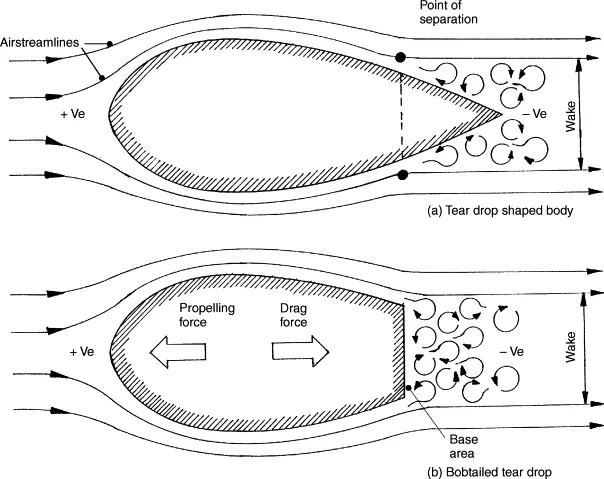
Q3. Explain the significance of the point of separation.
Ans:
- As the fluid flows around the surfaces it sticks to the surface forming the boundary layer.
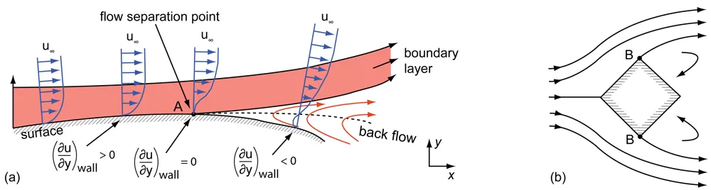
- When there is change in the curvature of the surface or the surface ends the flow detaches from the surface this point is known as point of seperation or seperation point.
- Here the flow below the detached boundary causes low pressure or inverse pressure gradient which starts to reverse the flow of the fluid.
- As there is low pressure or inverse pressure gradient the back surface experiences the suction from it resulting in increase in the overall drag effect.
- As the front part has high pressure and the end part has low pressure and there are irregularities in the wake region it causes buffeting, which may cause structural issues in the body.
- In aerodynamics when there is flow seperation it has two major negative impacts [1]:
- Pressure drag increases.
- And lift is reduced.
- In some cases the skin friction drag is reduced as there is no contact between the fluid and surface after point of seperation.
Conclusion:
- The simulation is run successfully for the external aerodynamic analysis over Ahmed body and the procedure and results clearly described.
- The simulation is run for three different cases of mesh elements sizes:
- Case-1: Outer enclosure = 80mm, Inner enclosure = 30mm, First layer thickness = 0.7mm, with 10 layers (0.3 million cells).
- Case-2: Outer enclosure = 75mm, Inner enclosure = 25mm, First layer thickness = 0.7mm, with 10 layers (0.5 million cells).
- Case-3: Outer enclosure = 60mm, Inner enclosure = 20mm, First layer thickness = 0.7mm, with 10 layers (1 million cells).
- As the mesh is refined the results get to more accurate side as there is very fine distribution of elements and helps in equal defining of initial conditions.
- All the Results with velocity, pressure contours and vectors with flow distribution graph are described for each case.
References:
- E.L. Houghton, P.W. Carpenter, Steven H. Collicott, Daniel T. Valentine,
Chapter 1 - Basic Concepts and Definitions,
Editor(s): E.L. Houghton, P.W. Carpenter, Steven H. Collicott, Daniel T. Valentine,
Aerodynamics for Engineering Students (Seventh Edition),
Butterworth-Heinemann,
2017,
Pages 1-86,
ISBN 9780081001943,
https://doi.org/10.1016/B978-0-08-100194-3.00001-8.
(https://www.sciencedirect.com/science/article/pii/B9780081001943000018) - Meile, Walter & Brenn, Günter & Reppenhagen, Aaron & Lechner, Bernhard & Fuchs, Anton. (2011). Experiments and numerical simulations on the aerodynamics of the Ahmed body. CFD Letters. 3.Meile, Walter & Brenn, Günter & Reppenhagen, Aaron & Lechner, Bernhard & Fuchs, Anton. (2011). Experiments and numerical simulations on the aerodynamics of the Ahmed body. CFD Letters. 3.