Week 8 - Simulating Cyclone separator with Discrete Phase Modelling

Aim: To study the effect of particle size and fluid velocity on the effeciency of the cyclone seperator using the numerical method.

Objective:

1. Import, clean and extract the geometry for the simulation.
2. Mesh the geometry using the cartesian system with appropriate named selections.
3. Setup the physics and boundary conditions for the model.
4. Run the simulation and analyze the effects of particle size and fluid velocity on the effeiceny of the cyclone seperator.

Theory:`

Some of the emphirical models used for the calculating the cyclone seperator efficieny along with brief description are given below:

1. Iozia and Leith Model:
   • This model is developed from the modification of Barth model.
   • According to this model there are two forces experienced by the particle:
     1. Centrifugal force.
     2. Flow resistance.
   • The trap/collection efficieny for diameter of the particle 'd' is calculated by:
     1. `ηi = 1 / (1 + (dpc)/(dp i)^beta)`
     2. were,
     3. `beta` is the slope expression derived from the experimental data of cyclone seperator with diameter of 0.25m.
     4. `beta = (0.62-0.87ln((dpc)/100)+5.21ln((ab)/(D^2))+(1.05[ln((ab)/D^2)]^2))`
     5. dpc is the 50% cut size given by Barth.
     6. `dpc = [( 9 *µ*Q )/(π*ρp* Zc*Vt^ 2max)]^0.5`
     7. Zc = core length.
     8. dc = core diameter.
2. Li and Wang Model:
   • This is the two dimensional analytical expression for the particle distribution in cyclone.
   • It include some of the major phenomenon occuring in the processor i.e. particle bounce and turbulent diffusion.
   • This is model is developed based on the following assumptions:
     1. The radial particle velocity and radila concentration profile are not constant for the oncollected particles within the cyclone.
     2. The boundary conditions in accordance with the turbulent diffusion co-efficient and particle bounce entrainment on the cyclone wall are:
        • c = c0, at `theta = 0`
        • `Dr((dc)/(dr)) = (1-alpha)omegac, at - r = D/2.`
     3. The tangential velocity is related to the radius of the cyclone as,
        • `uR^n = constant`
3. Koch and Licht Model:
   • This model describes the particle motion at the entry and coolection/trap region.
   • It recognized the inherent turbulence nature of the cyclone.
   • The distribution of gas residence time within the cyclone is taken into consideration.
   • There are certain assumptions for this model:
     1. The tamgential velocity of the particles is same as the gas tangentially velocity, i.e. there is no slip between the particle and the gas.
     2. The tangential velocity is dependent on the radius of the cyclone and is given by `uR^n = constant`
   • The efficiency according to this model can be calculated as:
     • `ηi = 1 − exp{ −2[(Gτi Q)/ (D3) (n + 1)]}^(0.5/(n+1))`
     • were,
     • `G = (8kc)/((ka)^2(kb)^2)` factor related to the cyclone configuration.
     • `n = 1 − { 1 − ((12D)^0.14)/ 2.5}{ (T + 460)/( 530)}^0.3` (n is related to the index)
     • `τi = ((ρp)*(d^2) p i)/( 18µ)` (`tau` is relaxation term)
4. Lapple Model:
   • This is the developed based on the force balance.
   • Here the flow resistance is neglected.
   • Here the assumption is that particles are equally spaced at the inlet.
   • The particles in the half width to the cyclone wall are collected with 50% efficiency.
   • The efficeny of collection is given by:
     • `ηi = 1/( 1 + ((dpc)/(d¯ p i))^2`
     • were,
     • dpc is the 50% cut diameter given by - `= [ (9 µb)/( 2π Ne * Vi(ρp − ρg)) ]^(1/2)`
     • Ne is the number of revolution.

Content of the body:

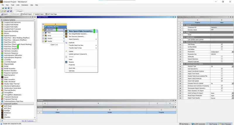
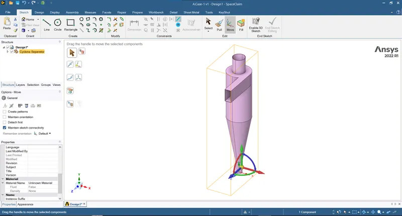
1. Open the Fluent module and imprt the geometry into the space claim (Drag and drop):
   1. 
   2. 
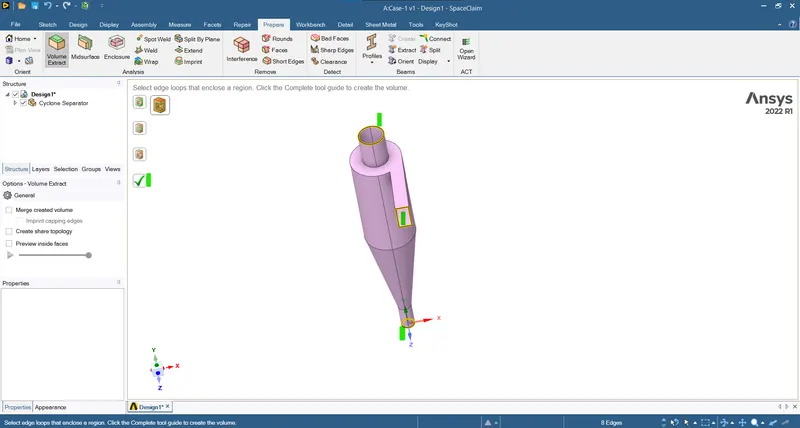
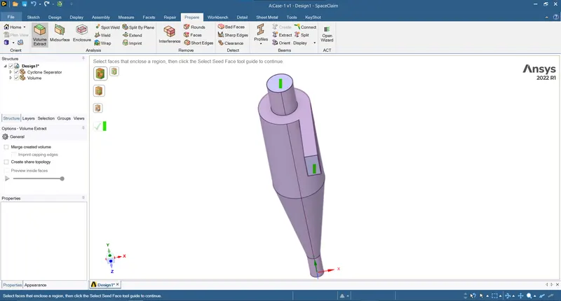
   3. Now extract the geometrical volume using the volume extract tool (Prepare > Extract volume > Select the edges > OK):
   4. 
   5. 
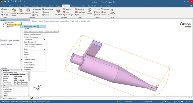
   6. We suppress the external geometry as we don't need the external geometry for the simulation (Selecet the geometry > Suppress the geometry):
   7. \
   8. 
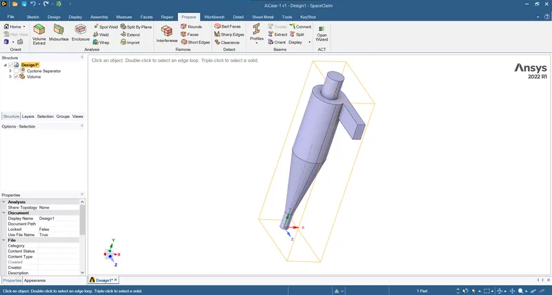
   9. The above geometry is used to run the simulations.
   10. Now as the geometry is clean and volumes are extracted we can proceed for meshing.
2. Meshing:
   1. 
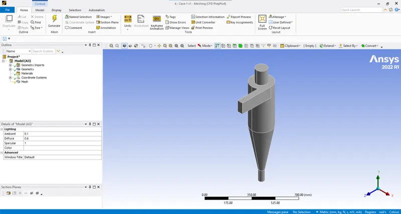
   2. Now generate the baseline default mesh to ensure there are no errors (Mesh > Generate mesh):
   3. 
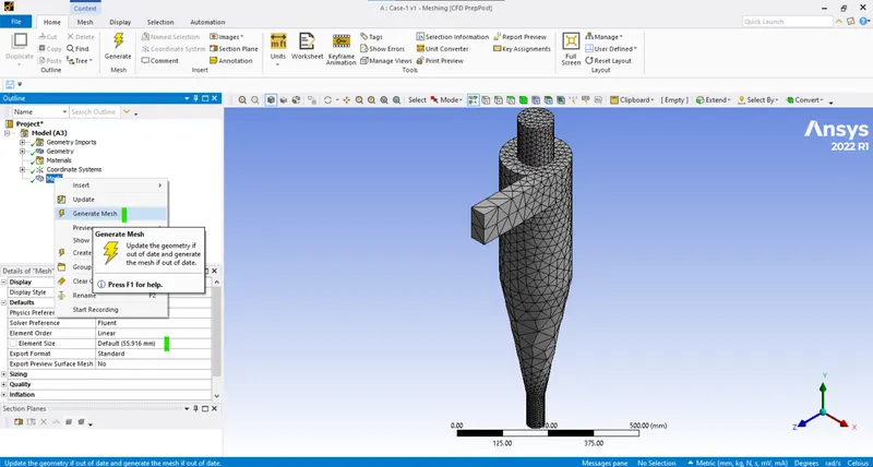
   4. Now as there are no errors or warnings we can proceed for the mesh refinement.
   5. For the geometry cntaining the swirls/spiral flows an cartesian mesh as it gives the better results for this kind of simulation compared to default element tria.
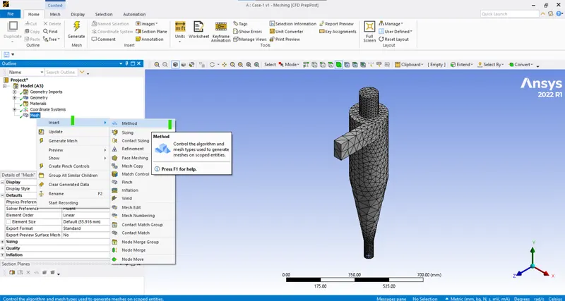
   6. To perform the cutcell meshing we need to add the cartesion method (Mesh > Method > Select the whole body > Cartesian):
   7. 
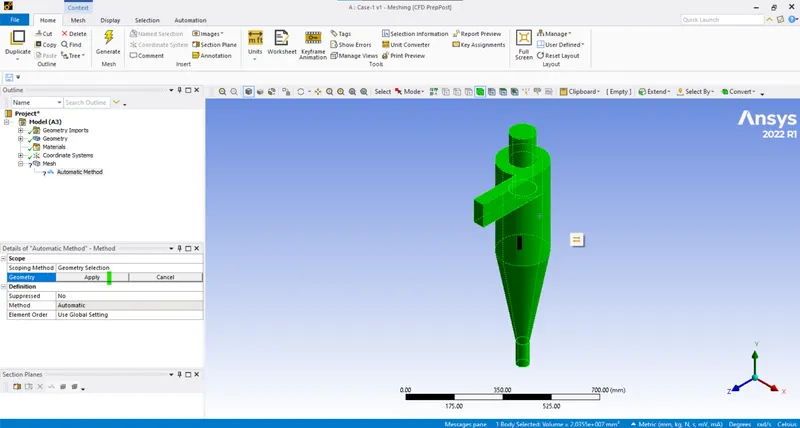
   8. Select the body > Apply:
   9. 
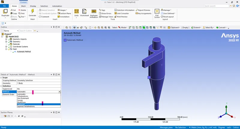
   10. Select the method to cartesian:
   11. 
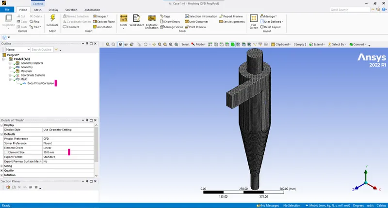
   12. Due to the larger element size we see a distorted mesh so changing the mesh size to lower size:
   13. 
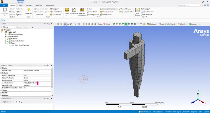
   14. After reducing the element size (10 mm):
   15. 
   16. Now naming the surfaces:
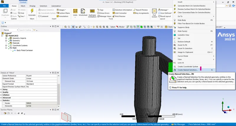
   17. Inlet (Select the surface > Create named selection):
   18. 
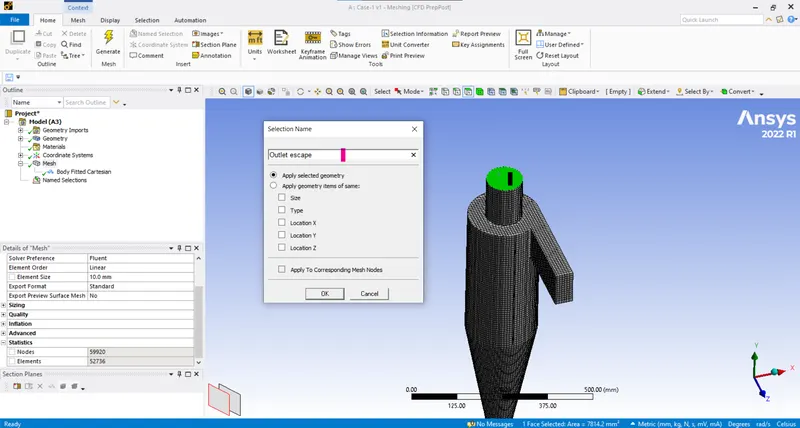
   19. Outlet escape:
   20. 
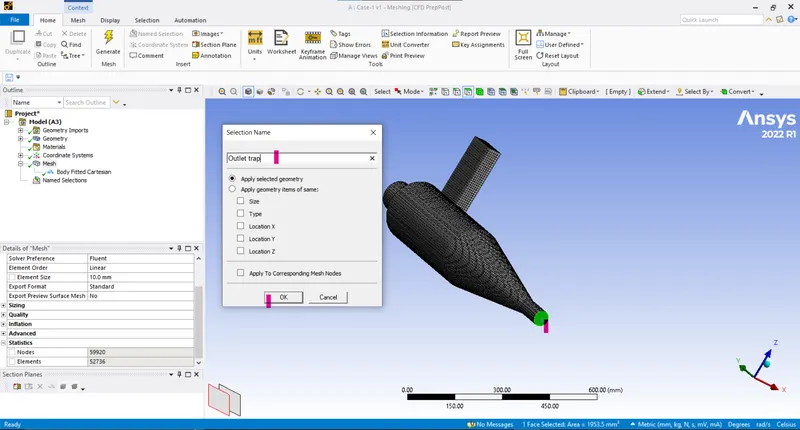
   21. Outlet trap:
   22. 
   23. Now updating the mesh conditions (Mesh > Update):
   24. 
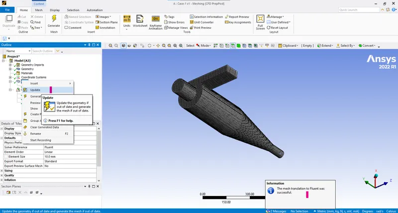
   25. Now the meshing and naming is complete we can proceed to the setup.
3. Setup:
   1. Here we define the boundary conditions and physics behind the simulation.
   2. Open the setup using the double precision and best number of processors:
   3. 
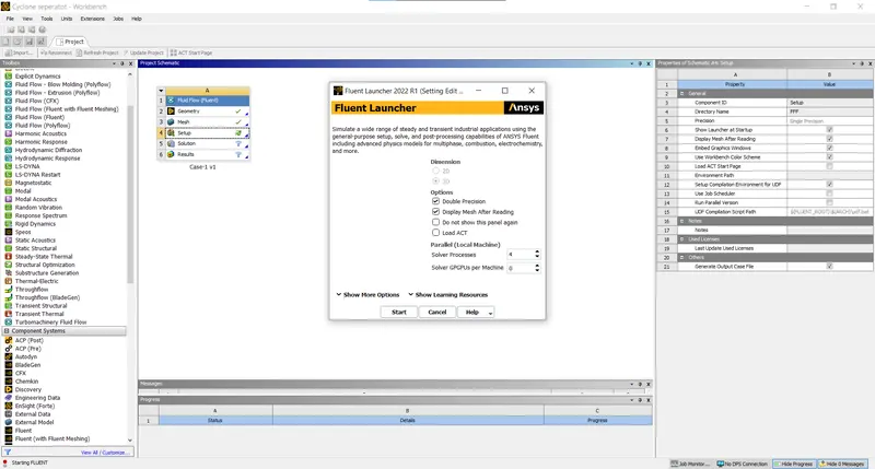
   4. Here enabling the gravity and viscous model as k-epsilon with RNG model as the model is suitable for the flow in which the swirling forces are dominating and enabling the swirl dominated flow in the RNG options:
   5. 
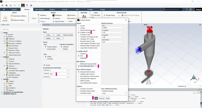
   6. Now setting up the discreate phase model:
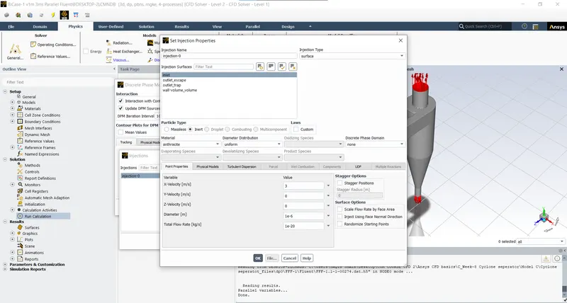
   7. As the particles are in continious interactions with the fluid carring it we should enable the Interaction with Continious Phase with update every 10 iterations.
   8. 
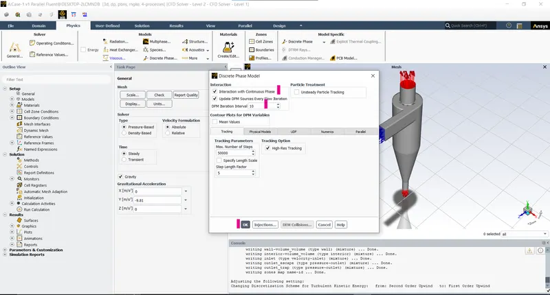
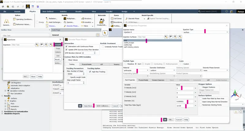
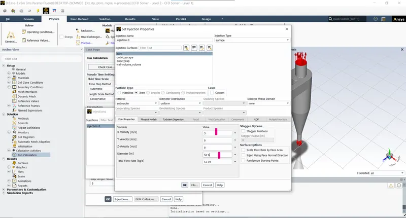
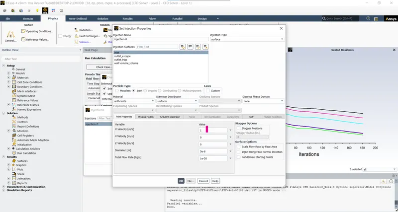
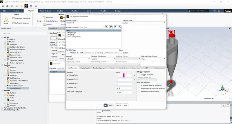
   9. Now defining up the injection parameters (Discreate phase model > Injection properties >Create):
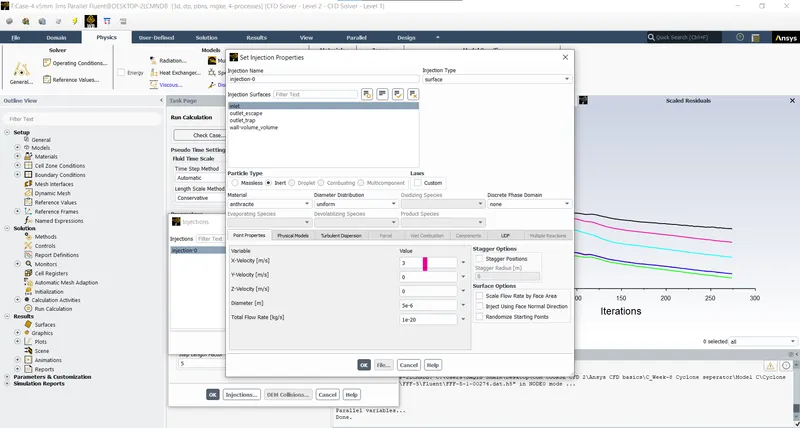
   10. Select the injection type as surface at the Inlet and define the velocity(3 m/s) and size of the particles (1micro) with anthracite as the material:
   11. 
   12. Now defing the boundary conditions:
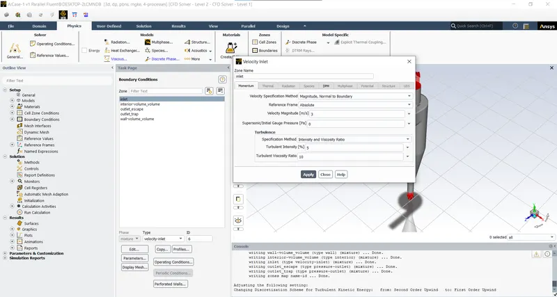
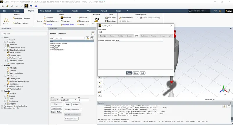
   13. Inlet - Velocity inlet (3m/s) and disreate phase boundary condition as reflect Physics > boundaries > > select the boundaries > define):
   14. Here reflect is selected because the surface must reflect the particles at the inlet, these values are defined for the main phase fluid.
   15. 
   16. 
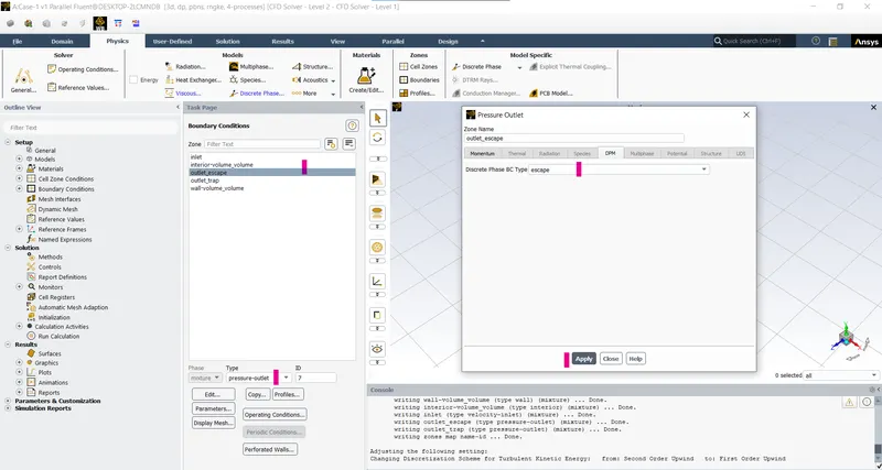
   17. Outlet escape: Select this outlet as the pressure outlet and the discreate phase boundary type as escape:
   18. 
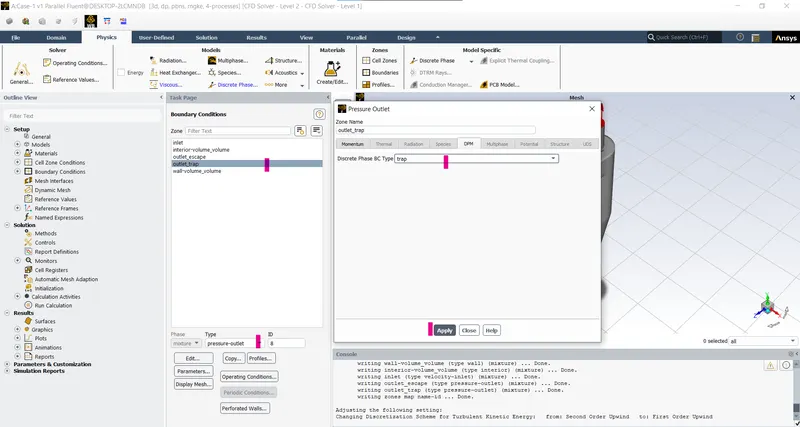
   19. Outlet trap: Select the outlet as pressure outlet and discreate phase boundary type as trap:
   20. \
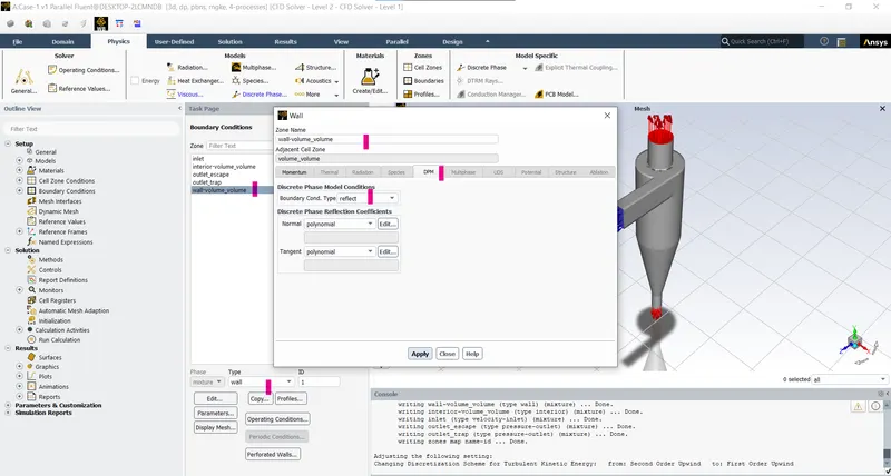
   21. Wall: Select as wall with Discreate phase boundary type as reflect:
   22. 
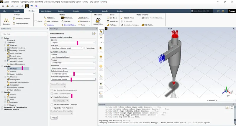
   23. In the methods second order Upwind is selected for better accuracy (Solution > Scheme-Coupled):
   24. 
   25. Initialization (Solution initialization > Standard initialization > Compute from Inlet > Initialize):
   26. 
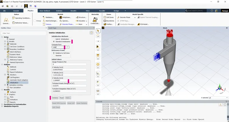
   27. The velocity given for the partivcles was in x-direction i.e. normal from the surface so, here the velocity is at negative z direction.
   28. Running the simulations for 500 iterations:
   29. 
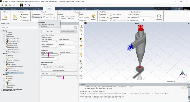
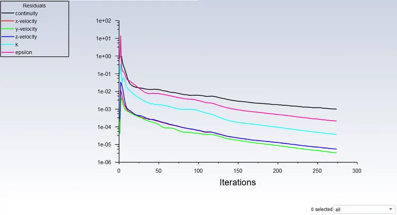
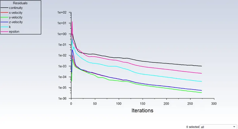
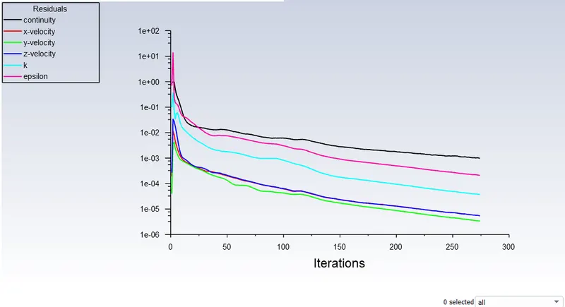
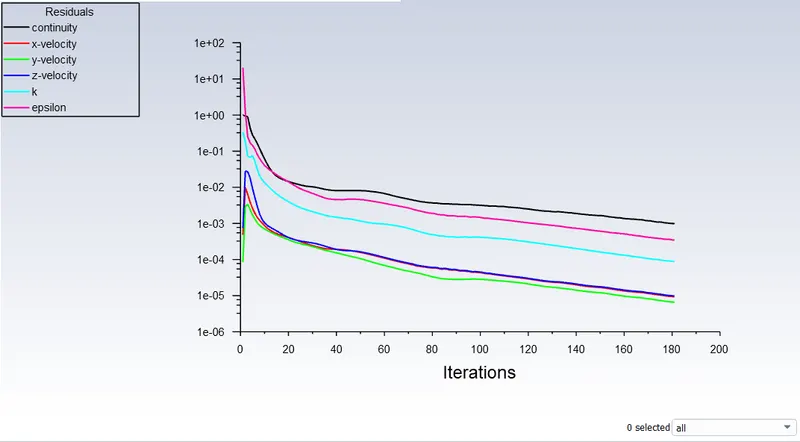
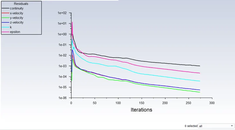
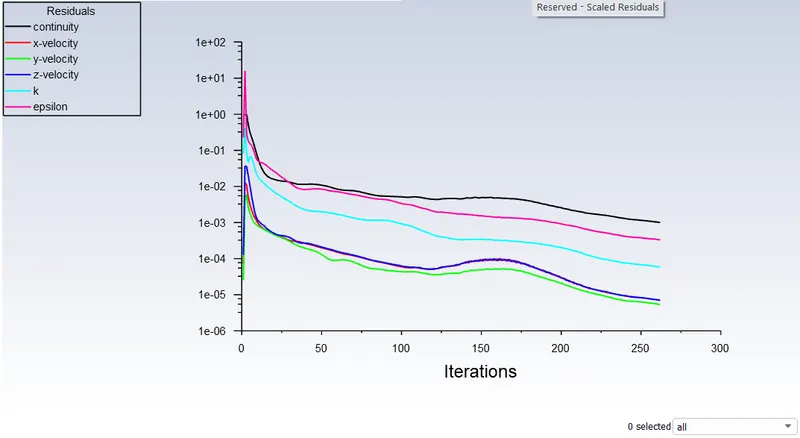
   30. The solution is converged after 178 iteration.
   31. 
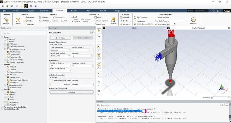
   32. Tracked particles - 91
   33. Escaped - 12
   34. Traped - 91
   35. Pressure difference at the inlet and the outlets (Total pressure) (Reports > Surface reports > Area-Weighted average > Pressure > Total pressure inlet and outlet escape):
   36. 
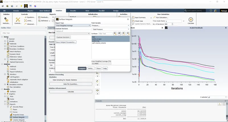
   37. Inlet pressure = 26.420039 Pa.
   38. Outlet escape = 3.5397838 Pa.
   39. Pressure difference = 22.8802552 Pa.
   40. Now saving the particles track data to import in the post processing (File > Export > Particle history data > Injection > Save):
   41. 
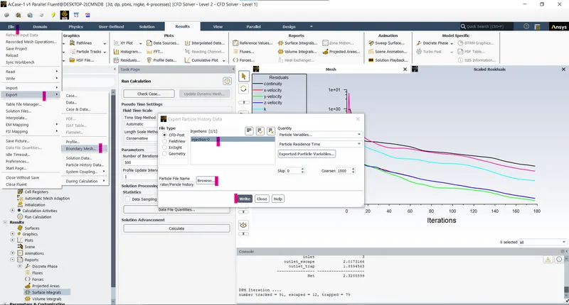
   42. Now as the solution is complete we can proceed to the post-processing.
4. Post-processing (Results):
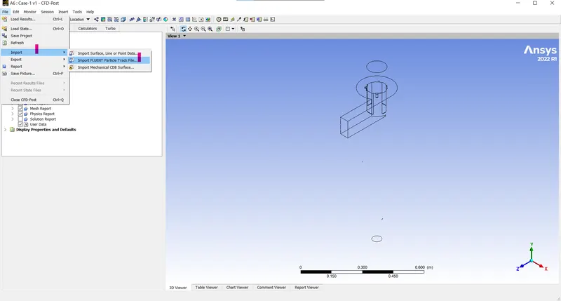
   1. Import the particle track history data (File > Import > Particle track file > select > Ok):
   2. 
   3. Toview the particle time of the anthracite particles (variable > Fluent PT Anthrasite > Injection > Anthrasite Particle time > Apply):
   4. 
   5. 
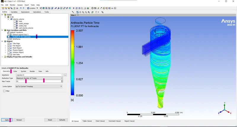
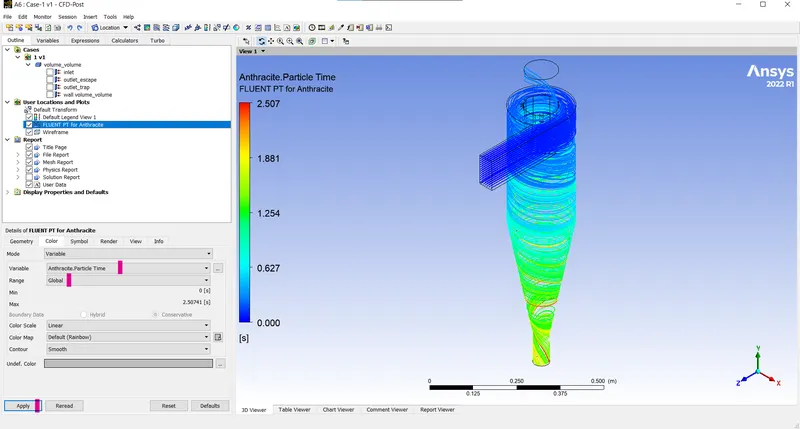
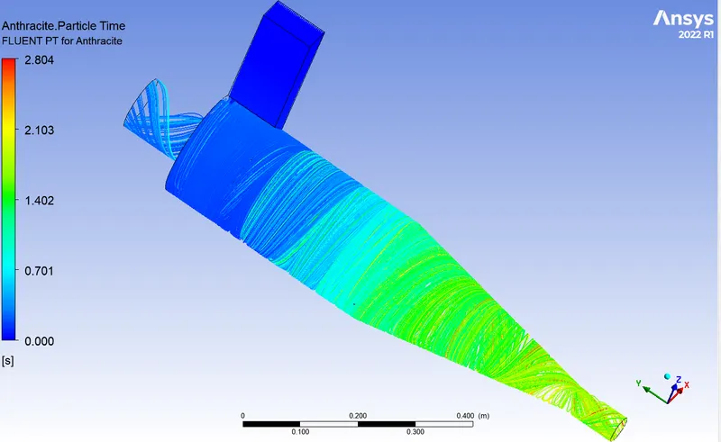
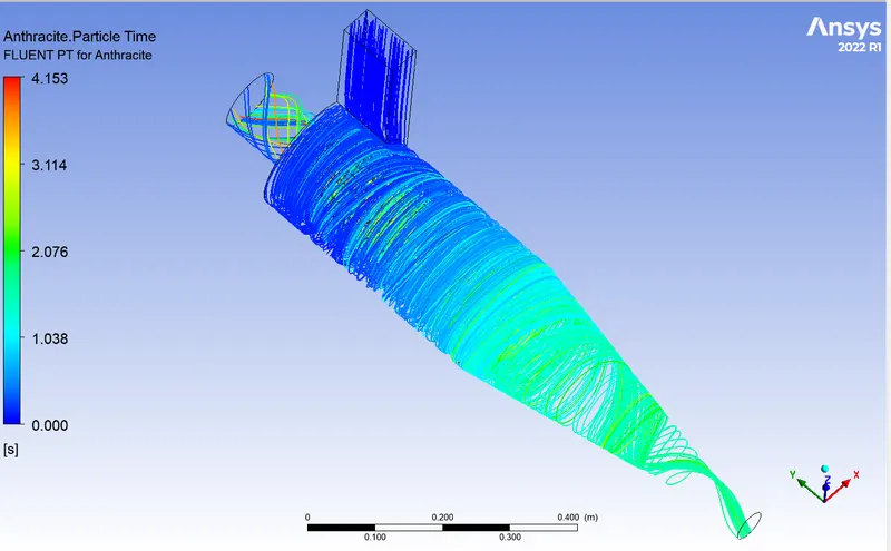
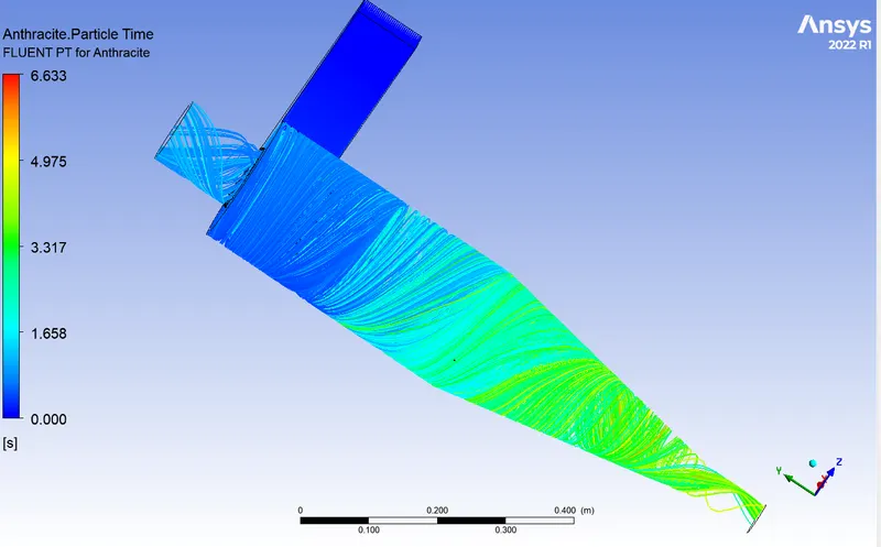
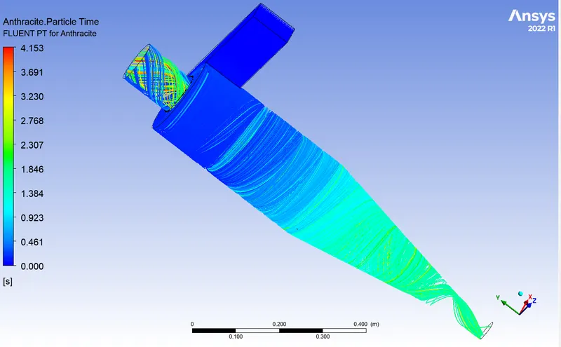
   6. The particle time shows the time taken by the particles to complete the flow and escape or trap.
   7. Here we can see the time taken by the anthrasite particles to escape or trap.
   8. The longest time taken is 2.507 seconds.
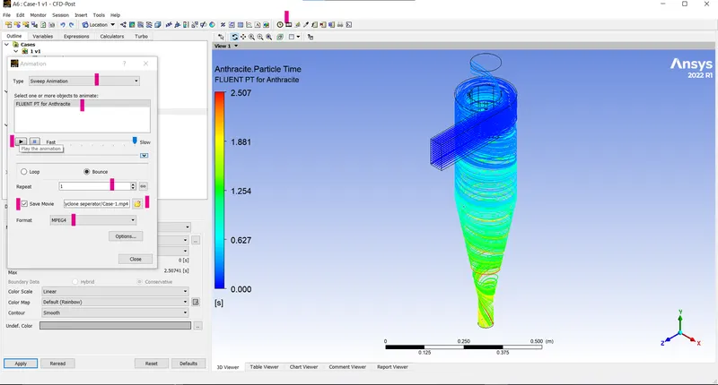
   9. Now creating the animated file to view the particle movement (Animation > Sweep animation > Anthrasite particle time > Save > Set frames > Play):
   10. 
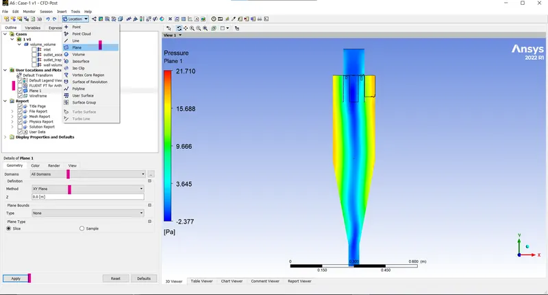
   11. To create the contours we should create plane (Location > Plane > XY plane > Variable > Apply):
   12. 
   13. Pressure contours:
   14. 
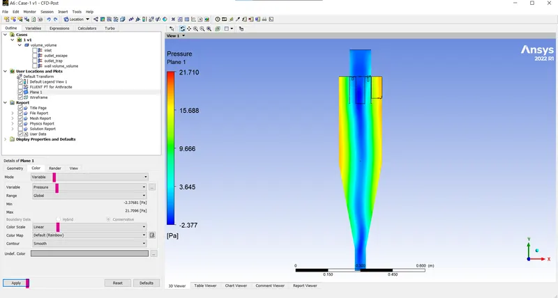
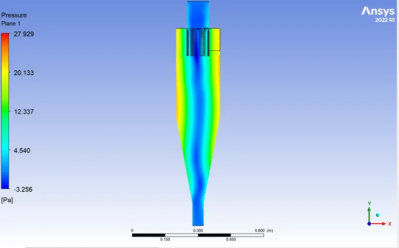
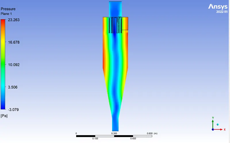
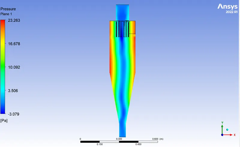
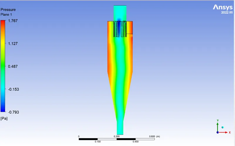
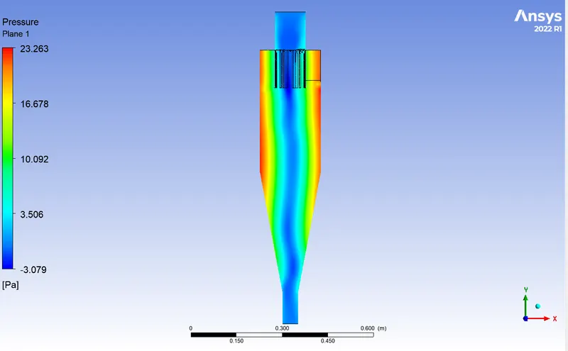
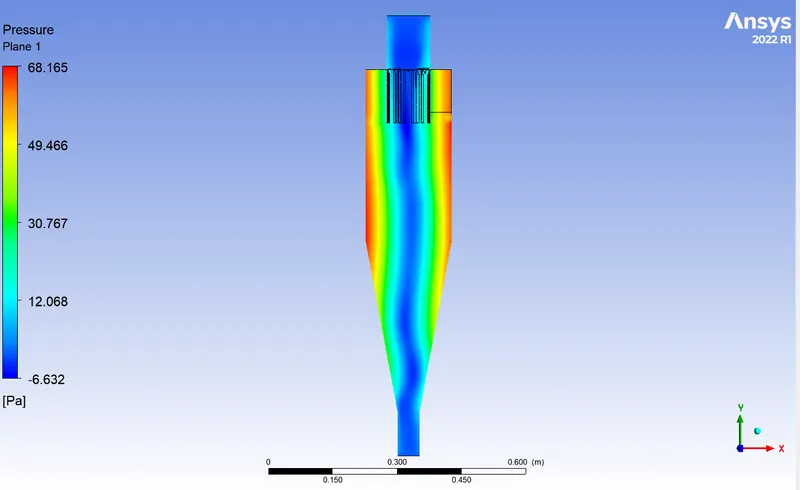
   15. Pressure contours represents the varaition of pressure accross the cyclone seperator, as we can see there due to the fluid entering tangentially to the body of the cyclone seperator the swirl action is created anwhich leads to the denser fluid region near the circumference of the body causing more pressure on the walls and there isnegative pressure in the centre.
   16. Velocity conoturs:
   17. 
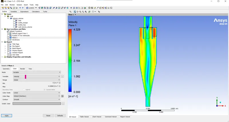
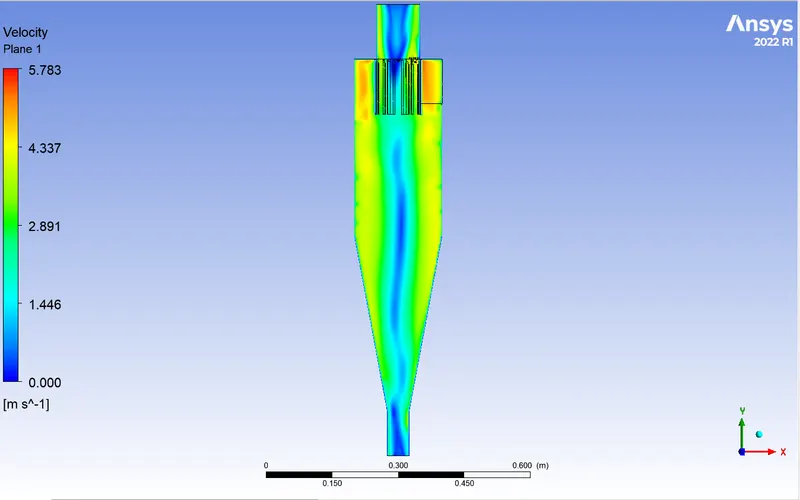
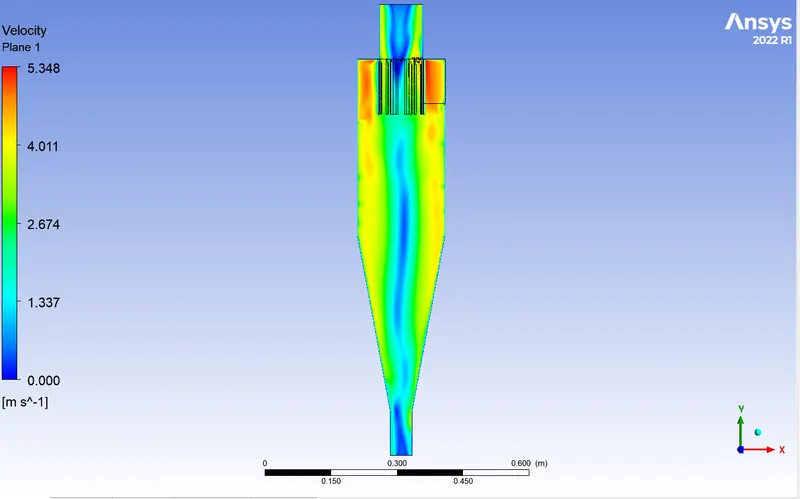
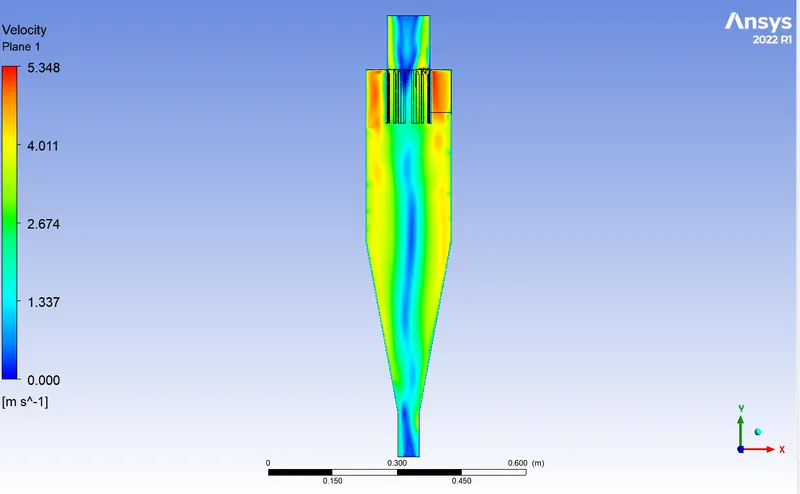
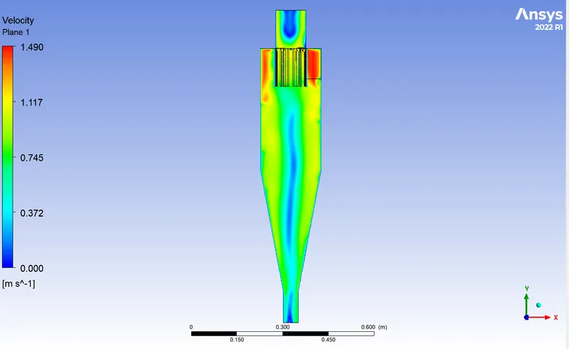
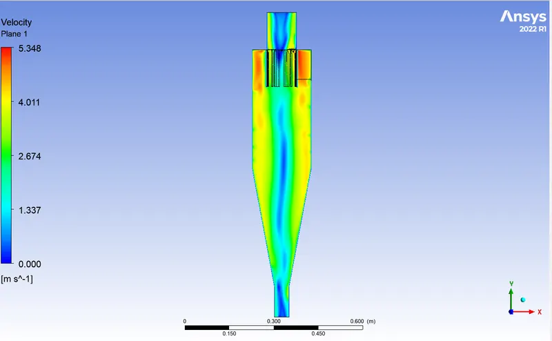
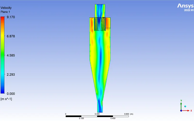
   18. The velocity contours represents the velocity variation accross the geometry, here we can observe that the fluid entering has the highest velocity compared to rest of the case.
   19. This is due to the flow slows done as there is no effort to increase the velocity as it proceeds.
   20. There is near still region in the centre of the cyclone (but some fluid particles may have high local rotation around there own axis) this is due the fact that most of the mass is flowing in the circular motion and are thrown in the outward direction due to the centrifugal forces and as we move to the centre of the circle the circumference of the circle decreases which indicates less displacement and thus less velocity.
   21. Now by changing the boundary conditions and particles size we can run the simulations for the cases described.
5. To calculate the efficiency:
   1. Efficiency = Particles Traped/Total particles

Results:

1. Mesh:
   1. 
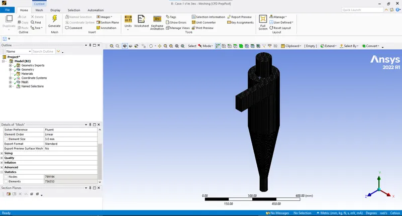
   2. Mesh count - 756353.
   3. Baseline mesh element size - 3mm.
2. Case-1:
   1. Residuals:
   2. 
   3. Velocity contours and streamlines:
   4. 
   5. Pressure contours and streamlines:
   6. 
   7. Particle Time:
   8. 
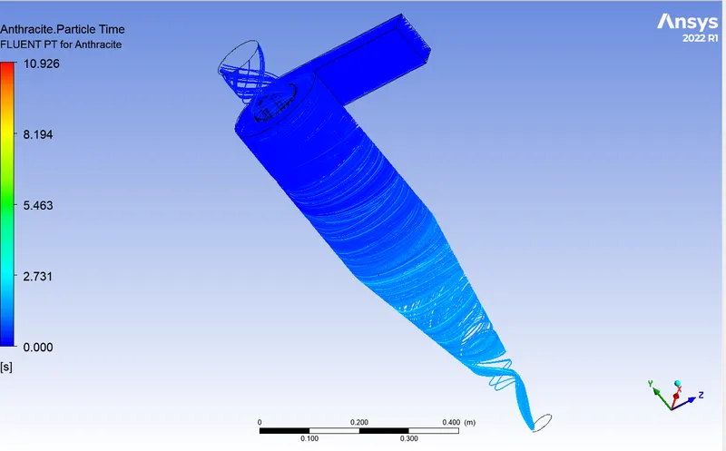
   9. The streamlines represents the particles motion in the fluid.
   10. This variations shows the particle time spent in the cyclone seperator.
3. Case-2:
   1. Residuals:
   2. 
   3. 
   4. Velocity contours and streamlines:
   5. 
   6. Pressure contours and streamlines:
   7. 
   8. Particle Time:
   9. 
4. Case-3:
   1. Residuals:
   2. 
   3. 
   4. Velocity contours and streamlines:
   5. 
   6. Pressure contours and streamlines:
   7. 
   8. Particle Time:
   9. 
5. Case-4:
   1. Residuals:
   2. 
   3. 
   4. Velocity contours and streamlines:
   5. 
   6. Pressure contours and streamlines:
   7. 
   8. Particle Time:
   9. 
6. Case-5:
   1. Residuals:
   2. 
   3. 
   4. Velocity contours and streamlines:
   5. 
   6. Pressure contours and streamlines:
   7. 
   8. Particle Time:
   9. 
7. Case-6:
   1. Residuals:
   2. 
   3. 
   4. Velocity contours and streamlines:
   5. 
   6. Pressure contours and streamlines:
   7. 
   8. Particle Time:
   9. 

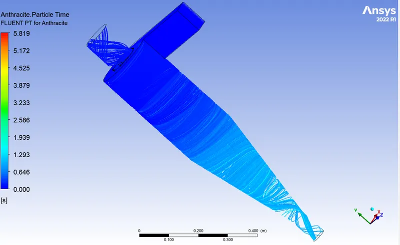
Table Contents:

Cases	Particle size (micrometer)	Velocity (m/s)	Total particles	Particles Escaped	Particles Traped	Efficiency (0-1)	Pressure Difference (Pascals)
Case-1	1	3	578	108	469	0.811419	27.6639965
Case-2	3	3	578	115	463	0.801038	27.6639965
Case-3	5	3	578	211	367	0.634948	27.6639965
Case-4	5	1	578	119	459	0.794118	2.38693686
Case-5	5	3	578	211	367	0.634948	27.6639965
Case-6	5	5	578	93	434	0.750865	79.6892230

Animations table:

Cases	Particle Time	Velocity	Pressure
Case-1	Particle Time	Velocity	Pressure streamline
Case-2	Particle Time	Velocity	Pressure streamline
Case-3	Particle Time	Velocity	Pressure streamline
Case-4	Particle Time	Velocity	Pressure Streamline
Case-5	Particle Time	Velocity	Pressure streamline
Case-6	Particle Time	Velocity	Pressure streamline

Conclusion:

1. The simulation is performed successfully with defined paramters and conditions.
2. In the first three case the Particle size is varied (1 micrometer to 5 micrometer) with constant velocity of 3 m/s.
3. In the next cases the velocity is varied (1m/s to 5 m/s) with constant element size (5 micrometer).
4. The effect of particle size and velocity on the motion behaviour and the effeciency of the cyclone seperator is stuided.
5. As the particle size increase the effeciency decreases.
6. This is due to the higher momentum gained due the higher mass which leads in more velocity to overcome the drag/frontal resistance to fall towards trap thus leads to the escape.
7. As the velocity increases the percentage of the incomplete particles increases which are stuck in circular motion inside the cyclone seperator.
8. As the velocity increases the pressure difference also increases very rapidly as it can said from the observation that pressure difference only depends on the velocity of the fluid not on the particle size.
9. The particle time, velocity streamline and pressure streamlines are reported in the form of video animations.

References:

1. Gimbun, Jolius & Luqman Chuah, Abdullah & Choong, TSY & Fakhru'l-Razi, A.. (2005). A CFD Study on the Prediction of Cyclone Collection Efficiency. International Journal for Computational Methods in Engineering Science and Mechanics. 6. 161-168. 10.1080/15502280590923649.
2. B. Wang, D.L. Xu, K.W. Chu, A.B. Yu,
   Numerical study of gas–solid flow in a cyclone separator,
   Applied Mathematical Modelling,
   Volume 30, Issue 11,
   2006,
   Pages 1326-1342,
   ISSN 0307-904X,
   https://doi.org/10.1016/j.apm.2006.03.011.
3. Liwang Wang, Erwen Chen, Liang Ma, Zhanghuang Yang, Zongzhe Li, Weihui Yang, Hualin Wang, Yulong Chang,
   Numerical simulation and experimental study of gas cyclone–liquid jet separator for fine particle separation,
   Chinese Journal of Chemical Engineering,
   Volume 51,
   2022,
   Pages 43-52,
   ISSN 1004-9541,
   https://doi.org/10.1016/j.cjche.2021.12.015.