Project 2 - Rankine cycle Simulator
Aim: To create a simulator of the Basic Rankine cycle by programming using Matlab.
Objectives:
- Understand the working of the Basic Rankine cycle.
- Write a program to simulate the basic Rankine cycle:
- Taking the input conditions from the users.
- Based on the input initial conditions calculate the state variables at each state (also intermediatory states).
- Then calculate the various performance factors using the state conditions.
- Plotting the Temperature-Entropy diagram and Enthalpy-Entropy diagram with appropriate labeling and title.
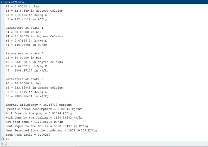
- Displaying the results in the command window.
Theory:
- The basic Rankine cycle is the idealized thermodynamic vapor power cycle.
- It describes the working of some heat engines.
- It explains extracting the heat from the fluid and converting it into work where the fluid travels from the heat source to the heat sink.
- Here the idealized/basic cycle represents the basic intended operation and neglects the unnecessary or real-time effects.
- The Rankine cycle has majorly four steps:
- 1-2 Isentropic expansion in the turbine.
- 2-3 Constant pressure heat rejection in the condenser.
- 3-4 Isentropic compression in the pump.
- 4-1 Constant pressure heat addition in the boiler.
- First the water is heated in the boiler at constant pressure till it reaches the desired properties and is converted to saturated or superheated vapor.
- Then the saturated or superheated vapor from the boiler outlet is supplied to the turbine inlet were it is expanded isentropically onto the turbine blades and the turbine output is converted into useful work and the expanded low-pressure steam is sent to the condenser inlet.
- After the constant pressure heat rejection in the condenser the steam turns to the saturated liquid and it is pumped to the boiler using the pump isentropically and this cycle continues.
- Entropy: It is the system's thermal energy per unit temperature, it is the energy that is unavailable to do work.
- Enthalpy: It is the property of the thermodynamic system which is the measure of the energy, it is the summation of the internal energy and the product of the pressure and volume.
- A typical representation of the Rankine cycle is as follows:
- For saturated vapor as inlet.
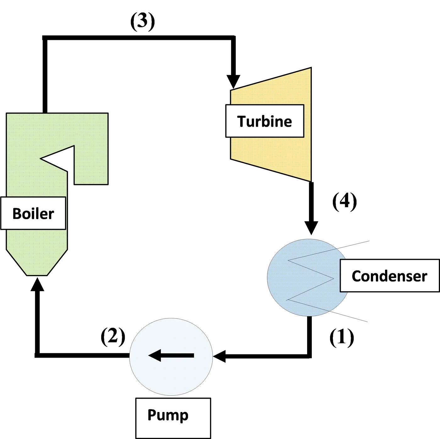
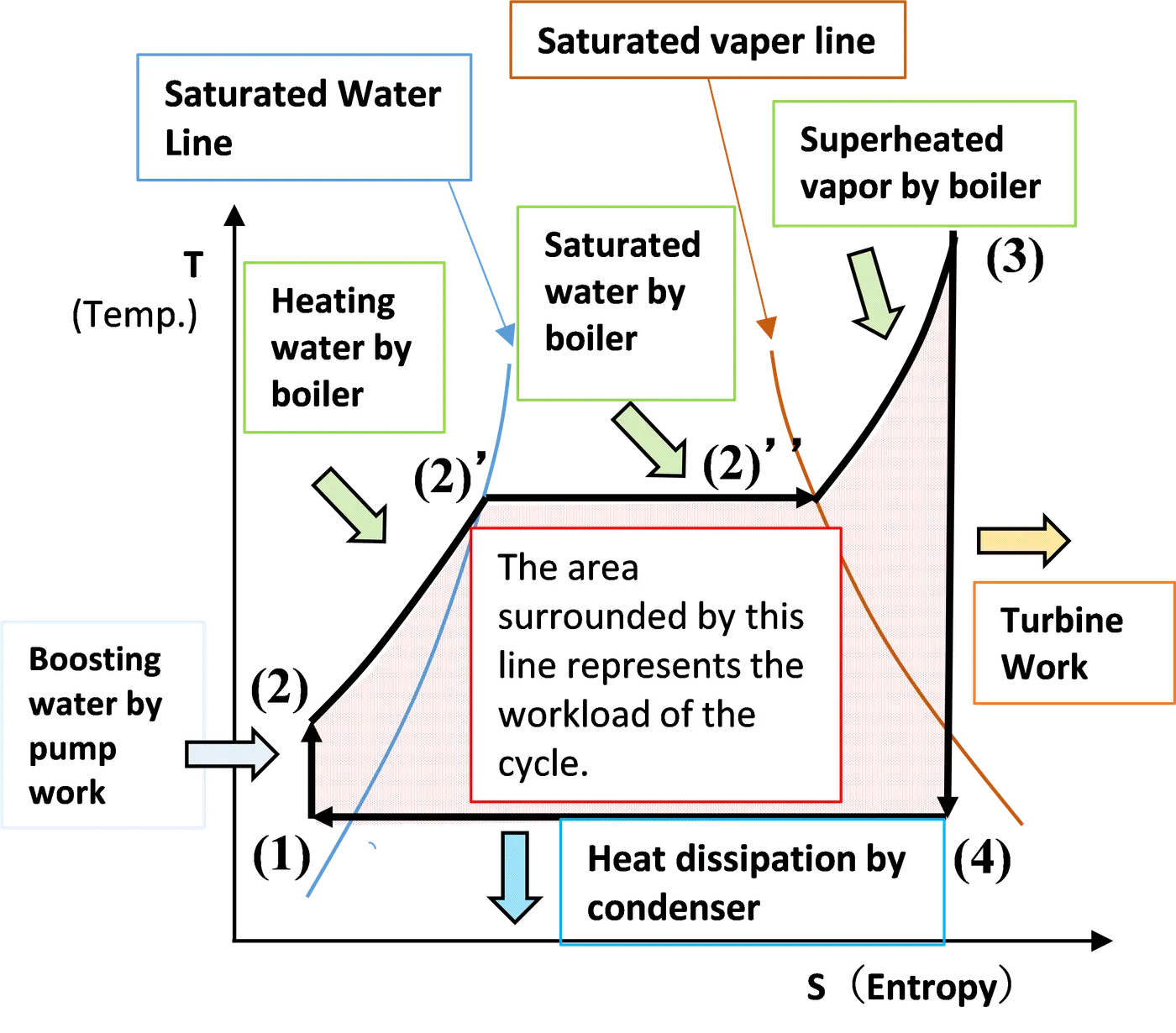
- T-S diagram of the Rankine cycle.
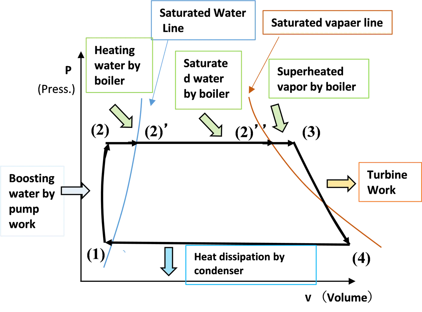
- P-V diagram of Rankine cycle.
- Basic Formulae:
- Work input to the pump (Wp or Win): It is the amount of energy(work) spent on the pump.
- Wp = v3*(p4-p3)*100 (kJ/kg).
- Work output from the turbine (WT): It is the amount of work obtained from the turbine.
- WT = h1 - h2 (kJ/kg).
- Heat added in the boiler (Qin): It is the heat added to the fluid in the boiler.
- Qin = h1-h4 (KJ/kg).
- Heat removed in the condenser (Qout): It is the amount of heat removed from the condenser
- Qout = h2 - h3 (KJ/kg).
- Thermal Efficiency: It is the ratio of net work obtained to the heat supplied.
- Thermal_Efficiency = ((Wnet)/(Qin))*100.
- Specific steam consumption (Con_sp): It is the mass flow rate of steam required to produce 1 kW of net work output.
- Con_sp = (3600)/(Wnet) kg/kWh.
- Net work output (Wnet): It is the work obtained after supplying energy to the pump.
- Wnet = WT - Win (kJ/kg).
- Back Work ratio: It is the ratio of the pump work to the turbine work.
- BWR = (Wp)/(WT).
- Work input to the pump (Wp or Win): It is the amount of energy(work) spent on the pump.
- Units:
- Temperature(T) in degrees Celsius.
- Pressure(p) in bars.
- Entropy(s) in kJ/Kg.K.
- Enthalpy(h) in kJ/kg.
- Thermal efficiency in percentage.
- Specific steam consumption in kg/kWh.
- Work done in kJ/kg.
- Heat added/rejected in KJ/kg.
- Abbreviations:
- Cv: Specific heat at constant volume.
- Cp: Specific heat at constant pressure.
- v: Saturated liquid volume.
Content of the body:
- The software used is Matlab.
- Clear all, close all and clc are used to clear the workspace variable, closing all the open windows if any, and clearing the command window respectively.
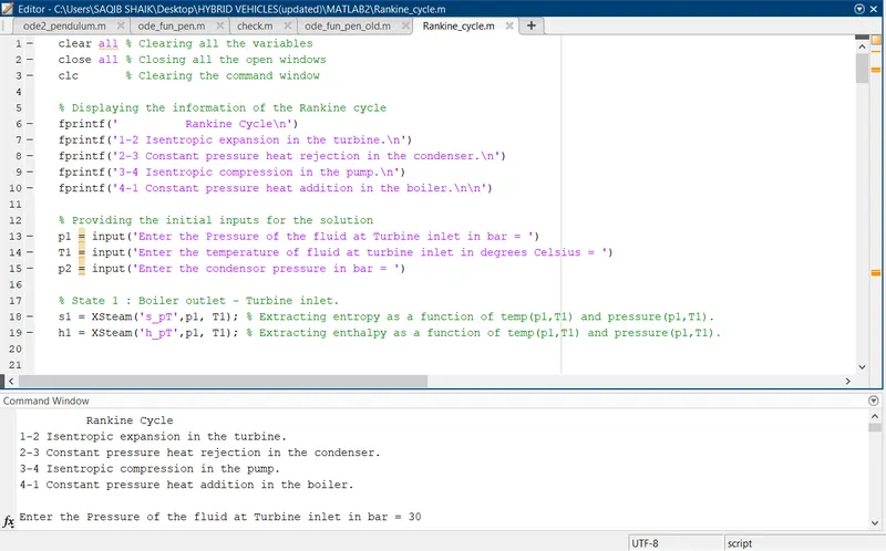
- The inputs are taken from the users using the 'input' command and stored in the variables as state 1 and 2 (as T1, p1 and p2) representing the temperature and pressure at state 1 and pressure at state 2.
- Now as we have the required data to begin the calculation for other parameters of the states we can start calculating the parameters at all the states.
- We need temperature, pressure, entropy and enthalpy at all the states.
- Note: There are only two operating pressure zones one from the boiler outlet till the turbine inlet(Boiler pressure p1) and the other after the turbine outlet till the boiler inlet(Condensor pressure p2).
- Now for state 1, we have the pressure (p1) and temperature (T1) so we need to calculate the enthalpy and entropy.
- State 1: (Turbine inlet/Boiler outlet)
- By using the XSteam function we can obtain the entropy and enthalpy at pressure (p1) and temperature (T1).
- s1 = XSteam('s_pT',p1, T1) Extracting the entropy by using the XSteam function specifying the property to be extracted as 's_pT' i.e. entropy at pressure p1 and temperature T1 and storing the output in variable s1.
- h1 = XSteam('h_pT',p1, T1) Extracting the enthalpy by using the XSteam function specifying the property to be extracted as 'h_pT' i.e. enthalpy at pressure p1 and temperature T1 and storing the output in variable h1.
- State 2: (Turbine outlet/Condensor inlet)
- Similar to state 1, we need the Temperature, entropy and enthalpy.
- Since the process 1-2 is isentropic entropy at state 1 and state 2 (s1 and s2) are equal.
- Now for the calculation of the enthalpy:
- Since the enthalpy needs to be calculated at the non-saturated region we need to first calculate the dryness fraction and then calculate the enthalpy at state 2:
- For the calculation of the dryness fraction the entropy at the saturated liquid and saturated vapor states are extracted using the sf2 = XSteam('sL_p', p2) and sg2 = XSteam('sV_p', p2) command (i.e. entropy at saturated liquid and saturated vapor state as a function of pressure) and storing in variables sf2 and sg2 respectively.
- By using the formula x = (s2-sf2)/(sf2-sg2) [simplification of s2 = sf2 + (x*(sf2-sg2))] we can calculate the dryness fraction.
- Now extracting the enthalpy at saturated liquid and saturated vapor/gas as a function of pressure at state 2 using the 'hf2 = XSteam('hL_p', p2)', 'hg2 = XSteam('hV_p', p2) ' and storing in hf2 and hg2 respectively.
- Now by using the formula 'h2 = hf2 + (x*(hf2-hg2))' we calculate the enthalpy at state 2.
- State 3: (Condensor outlet/Pump inlet):
- State 3 represents the fluid exiting the condenser and entering the boiler.
- Here the pressure is the same as condenser pressure as the pressure remains the same at the heat rejection and pumping state.
- Since we have the pressure at state 3 we can easily calculate the entropy and enthalpy using the 's3 = XSteam('sL_p', p3)' and 'h3 = XSteam('hL_p', p3)' respectively and storing them in 's3' and 'h3' respectively (i.e. entropy and enthalpy at the saturated liquid curve as a function of pressure because the condenser output is liquid).
- And as the condenser causes the phase change only and not in the temperature so, the temperature at state 2 and state 3 are equal (Any point beyond the saturated liquid curve the heat addition or rejection results in phase change only not the temperature till the saturated vapor curve).
- State 4: (Pump outlet/Boiler inlet):
- In pump at state 3-4 the isentropic compression occurs so the entropy is constant (s3 = s4).
- Since the pump is used for the liquids which are nearly incompressible the volume doesn't change much and in the boiler, heat is added at constant pressure and expanded at the turbine at the same pressure so, the pressure at state 4 and state 1 are the same.
- Since the work is done on the fluid the enthalpy at state 4 will be the summation of the pump work(Wp) and enthalpy at state 3, i.e. 'h4 = Wp + h3'.
- The work done on the pump is calculated by the formula 'Wp = v3*(p4-p3)*100' (units conversion is done).
- The Saturated liquid volume at state 3 needs to be calculated for the calculation of the work done on the pump, it;'s extracted by using the 'v3 = XSteam('vL_p', p3)' command i.e. specific volume at pressure state 3.
- Now for the calculation of the temperature at state 4 we use the relation 'T4 = T3/((p3/p4)^((K-1)/K))' to calculate where the 'k' is the ratio of the specific heat at constant pressure to specific heat at constant volume at state 4 (K = Cp4/Cv4).
- We have the temperature, entropy, enthalpy, and pressure at state 4.
- State 5 and 6 (Intermediate states during the boiling):
- State 5 and state 6 are the intermediate stages from the boiler inlet (state 4) to the turbine inlet (state 1).
- State 5 and state 6 are at the saturated liquid and saturated vapor lines.
- Entropy and enthalpy are calculated at the saturated liquid line as a function of pressure at state 1 (s5 = XSteam('sL_p',p1), h5 = XSteam('hL_p', p1) and stored in the variables as s5 and h5 respectively.
- Since state 5 is on the saturated liquid line and state 6 is at the saturated vapor line the temperature doesn't change as the phase change occurs due to latent heating so, the temperature at state 5 and state 4 are the same and is extracted from the library as 'T5 = XSteam('Tsat_p',p1)' as a function of pressure at state 1.
- The entropy and enthalpy are calculated at the saturated vapor line and are extracted from the library as 's6 = XSteam('sV_p',p1), h6 = XSteam('hV_p', p1)' and stored in 's6' and 'h6' respectively as a function of pressure at state 1.
- Now we have all the data to calculate the Thermal efficiency, Heat added in the boiler, Heat rejected in the condenser, Work done by the turbine, Work done on the pump, Net work done and specific steam consumption.
- Heat added (Qin) in the boiler at constant pressure (4-1):
- Formula: Qin = h1-h4, in KJ/kg.
- Heat rejected (Qout) in the condenser (2-3):
- Formula: Qout = h2 - h3, in KJ/kg.
- Work done on the pump (Win or Wp) (3-4):
- Formula: Wp = v3*(p4-p3)*100 or Wp = h4 - h3, in kJ/kg.
- This is the work supplied or done on the pump per kilogram.
- Work done by the turbine (WT) (1-2):
- Formula: WT = h1 - h2, in kJ/kg.
- This is the work output by the turbine per kilogram of steam flow.
- Net work done (Wnet):
- Formula: Wnet = WT - Win, in kJ/kg.
- Thermal efficiency:
- Thermal_Efficiency = ((Wnet)/(Qin))*100, in percentage.
- Specific steam consumption(Con_sp):
- Con_sp = (3600)/(Wnet), in kg/kWh.
- It is the amount of steam flow rate required to produce the 1 kW of net work.
- Back Work ratio: It is the ratio of the pump work to the turbine work.
- BWR = (Wp)/(WT).
- Program:
-
clear all % Clearing all the variables close all % Closing all the open windows clc % Clearing the command window % Providing the initial inputs for the solution p1 = input('Enter the Pressure of the fluid at Turbine inlet in bar = ') T1 = input('Enter the temperature of fluid at turbine inlet in degrees Celsius = ') p2 = input('Enter the condensor pressure in bar = ') % State 1 : Boiler outlet - Turbine inlet. s1 = XSteam('s_pT',p1, T1); % Extracting entropy as a function of temp(p1,T1) and pressure(p1,T1). h1 = XSteam('h_pT',p1, T1); % Extracting enthalpy as a function of temp(p1,T1) and pressure(p1,T1). % State 2 : Turbine outlet - Condensor inlet. s2 = s1; sf2 = XSteam('sL_p', p2); % Extracting entropy as a function of pressure(p2) at saturated liquid. sg2 = XSteam('sV_p', p2) ; % Extracting entropy as a function of pressure(p2) at saturated vapour. x = (s2-sf2)/(sf2-sg2); % Calculating the dryness fraction at state 2. hf2 = XSteam('hL_p', p2); % Extracting enthalpy as a function of pressure(p2) at saturated liquid. hg2 = XSteam('hV_p', p2) ; % Extracting enthalpy as a function of pressure(p2) at saturated vapour. h2 = hf2 + (x*(hf2-hg2)); % Calculating the enthalpy at state 2. % State 3 : Condensor outlet - Pump inlet. p3 = p2; % Pressure is same as the condensor pressure. s3 = XSteam('sL_p', p3); % Extracting the entropy as a function of pressure at state 3. h3 = XSteam('hL_p', p3); % Extracting the enthalpy as a function of pressure at state 3. % State 4 : Pump outlet - Boiler inlet. s4 = s3; % Isentropic compression process 3-4. p4 = p1; % equal pressure at boiler to turbine inlet. v3 = XSteam('vL_p', p3); % Extraction the specific volume at point 3. Wp = v3*(p4-p3)*100; % Calculating the workdone on the pump and correcting/converting the units. h4 = Wp + h3; % Calculating the enthalpy at point 4. % Heat added to the system (Boiler): Qin = h1-h4; % Work done by the turbine: WT = h1 - h2; % Heat removed from the system at condensor: Qout = h2 - h3; % Work done on the pump: Wp; % Net work done: Win = Wp; Wnet = WT - Win; % Thermal efficiency of the Rankine cycle. Thermal_Efficiency = ((Wnet)/(Qin))*100; % Specific steam consumption % Specific steam consumption (Con_sp) = (Mass flow rate of the steam)/(Net % work done) % Assuming that mass flow rate is in kg/sec we are converting it into % kg/hr by multiplying 3600. Con_sp = (3600)/(Wnet); % Calculating the Back work ratio (BWR): BWR = (Wp)/(WT); % In process 2-3 phase change occurs and temperature remains constant as T2 and T3 are equal T2 = XSteam('Tsat_p', p2); T3 = T2; % For the calculation at the point 4 we need to use the isentropic relation Cp4 = XSteam('Cp_ps',p4,s4); Cv4 = XSteam('Cv_ps',p4,s4); K = Cp4/Cv4; T4 = T3/((p3/p4)^((K-1)/K)); % Calculating the parameters at state 5 and 6 T5 = XSteam('Tsat_p',p1); s5 = XSteam('sL_p',p1); h5 = XSteam('hL_p', p1); T6 = T5; s6 = XSteam('sV_p',p1); h6 = XSteam('hV_p', p1); % Displaying the information of the Rankine cycle fprintf(' Rankine Cycle\n') fprintf('1-2 Isentropic expansion in the turbine.\n') fprintf('2-3 Constant pressure heat rejection in the condenser.\n') fprintf('3-4 Isentropic compression in the pump.\n') fprintf('4-5 Constant pressure heat addition in the boiler.\n\n') fprintf(' Inputs\n') fprintf('Turbine inlet temperature is %0.3f degrees Celsius\n', T1) fprintf('Turbine inlet pressure is %.3f bars\n', p1) fprintf('Condensor pressure is %0.3f bars\n\n', p2) % Displaying the results in the command window fprintf(' Results\n') fprintf('Parameters at state 1\n') fprintf('P1 = %.5f in bar\n', p1) fprintf('T1 = %.5f in degree celcius\n', T1) fprintf('S1 = %.5f in kJ/Kg.K\n', s1) fprintf('h1 = %.5f in kJ/kg\n\n', h1) fprintf('Parameters at state 2\n') fprintf('P2 = %.5f in bar\n', p2) fprintf('T2 = %.5f in degree celcius\n', T2) fprintf('S2 = %.5f in kJ/Kg.K\n', s2) fprintf('h2 = %.5f in kJ/kg\n\n', h2) fprintf('Parameters at state 3\n') fprintf('P3 = %.5f in bar\n', p3) fprintf('T3 = %.5f in degrees Celsius\n', T3) fprintf('S3 = %.5f in kJ/Kg.K\n', s3) fprintf('h3 = %.5f in kJ/kg\n\n', h3) fprintf('Parameters at state 4\n') fprintf('P4 = %.5f in bar\n', p4) fprintf('T4 = %.5f in degrees Celsius\n', T4) fprintf('S4 = %.5f in kJ/Kg.K\n', s4) fprintf('h4 = %.5f in kJ/kg\n\n', h4) fprintf('Parameters at state 5\n') fprintf('P5 = %.5f in bar\n', p1) fprintf('T5 = %.5f in degree celcius\n', T5) fprintf('S5 = %.5f in kJ/Kg.K\n', s5) fprintf('h5 = %.5f in kJ/kg\n\n', h5) fprintf('Parameters at state 6\n') fprintf('P6 = %.5f in bar\n', p1) fprintf('T6 = %.5f in degree celcius\n', T6) fprintf('S6 = %.5f in kJ/Kg.K\n', s6) fprintf('h6 = %.5f in kJ/kg\n\n', h6) fprintf('Thermal Efficiency = %.5f percent \n', Thermal_Efficiency) fprintf('Specific steam consumption = %.5f kg/kW\n', Con_sp) fprintf('Work Done on the pump = %.5f kJ/kg \n' , Win) fprintf('Work Done by the Turbine = %0.5f kJ/kg\n', WT) fprintf('Net Work done = %.5f kJ/kg \n', Wnet) fprintf('Heat input to the Boiler = %.5f in KJ/kg\n', Qin) fprintf('Heat Rejected from the condensor = %.5f KJ/kg\n', Qout) fprintf('Back work ratio = %.5f\n', BWR) % Extracting the data at saturated states and forming an array Ts = linspace(1,560,1000); for i = 1: length(Ts) ssl(i) = XSteam('sL_T', Ts(i)); % Entropy of saturated liquid at Temp T ssv(i) = XSteam('sV_T', Ts(i)); % Entropy of saturated vapour at Temp T hsl(i) = XSteam('hL_T', Ts(i)); % Enthalpy of saturated liquid at Temp T hsv(i) = XSteam('hV_T', Ts(i)); % Enthalpy of saturated vapour at Temp T end %Plotting the saturation line for plotting the cycle figure(1) plot(ssl, Ts, 'linewidth', 2); % Saturated liquid curve(T-S) hold on; % To hold the above curve for further plotting plot(ssv, Ts, 'linewidth', 2); % Saturated vapour curve(T-S) xlabel('Entropy (kJ/kg-k)'); % X label ylabel('Temperature (Degrees celsius)'); % y label title('Temperature v/s Entropy'); % Title of the graph % legend('Saturation curve') % Plotting the Rankine cycle process on the above curves plot([s1 s2], [T1,T2], 'linewidth', 2); % Isentropic expansion plot([s2 s3], [T2 T3], 'linewidth', 2); % Constant pressure heat rejection in the condensor plot([s3 s4], [T3 T4], 'linewidth', 2); % Isentropic compression % plot([s4 s5], [T4 T5]) % plot([s5 s6], [T5 T6]) % plot([s6 s1], [T6 T1]) plot([s4 s5 s6 s1], [T4 T5 T6 T1],'linewidth', 2); % Heat addition at constant pressure in boiler % Pointing the states text(s1+0.25, T1, '1'); % Pointing all the processes text(s2+0.25, T2, '2'); text(s3-0.25, T3, '3'); text(s4-0.25, T4+5, '4'); text(s5-0.25, T5+0.5, '5'); text(s6-0.1, T6+30, '6'); axis([0 10 0 T1+50 ]) % Providing the legends for the curves legend('Saturation Curve', 'Saturation Curve', 'Isentropic Expansion' , 'Isochoric Heat rejection', 'Isentropic Compression' , 'Isochoric Heat addition') % Plotting the Enthalpy-Entropy diagram figure(2) % Creating the second figure. plot(ssl, hsl); % Saturated liquid curve(S-H) hold on; % Holds the curve plotted in a single graph plot(ssv, hsv); % Saturated vapour curve(S-H) xlabel('Entropy (kJ/kg-k)'); % X label ylabel('Enthalpy (kJ/kg)'); % Y label title('Enthalpy v/s Entropy');% Title of the figure legend('Saturation curve'); % Adding the legends to the curves % Plotting the Rankine cycle process on the above curves plot([s1 s2], [h1,h2], 'linewidth', 2); % Isentropic expansion plot([s2 s3], [h2 h3], 'linewidth', 2); % Constant pressure heat rejection in the condensor plot([s3 s4], [h3 h4], 'linewidth', 2); % Isentropic compression plot([s4 s5], [h4 h5], 'linewidth', 2); % Heat addition at constant pressure in boiler plot([s5 s6], [h5 h6], 'linewidth', 2); % Heat addition at constant pressure in boiler plot([s6 s1], [h6 h1], 'linewidth', 2); % Heat addition at constant pressure in boiler % Pointing the states text(s1+0.25, h1, '1') text(s2+0.25, h2, '2') text(s3, h3-100, '3') text(s4, h4+180, '4') text(s5, h5+150, '5') text(s6, h6+150, '6') legend('Saturation Curve', 'Saturation Curve', 'Isentropic Expansion' , 'Isochoric Heat rejection', 'Isentropic Compression' , 'Isochoric Heat addition', 'Isochoric Heat addition', 'Isochoric Heat addition') - Final program:
-
clear all % Clearing all the variables close all % Closing all the open windows clc % Clearing the command window % Displaying the information of the Rankine cycle fprintf(' Rankine Cycle\n') fprintf('1-2 Isentropic expansion in the turbine.\n') fprintf('2-3 Constant pressure heat rejection in the condenser.\n') fprintf('3-4 Isentropic compression in the pump.\n') fprintf('4-1 Constant pressure heat addition in the boiler.\n\n') % Providing the initial inputs for the solution p1 = input('Enter the Pressure of the fluid at Turbine inlet in bar = ') T1 = input('Enter the temperature of fluid at turbine inlet in degrees Celsius = ') p2 = input('Enter the condensor pressure in bar = ') % State 1 : Boiler outlet - Turbine inlet. s1 = XSteam('s_pT',p1, T1); % Extracting entropy as a function of temp(p1,T1) and pressure(p1,T1). h1 = XSteam('h_pT',p1, T1); % Extracting enthalpy as a function of temp(p1,T1) and pressure(p1,T1). % State 2 : Turbine outlet - Condensor inlet. s2 = s1; sf2 = XSteam('sL_p', p2); % Extracting entropy as a function of pressure(p2) at saturated liquid. sg2 = XSteam('sV_p', p2) ; % Extracting entropy as a function of pressure(p2) at saturated vapour. x = (s2-sf2)/(sf2-sg2); % Calculating the dryness fraction at state 2. hf2 = XSteam('hL_p', p2); % Extracting enthalpy as a function of pressure(p2) at saturated liquid. hg2 = XSteam('hV_p', p2) ; % Extracting enthalpy as a function of pressure(p2) at saturated vapour. h2 = hf2 + (x*(hf2-hg2)); % Calculating the enthalpy at state 2. % State 3 : Condensor outlet - Pump inlet. p3 = p2; % Pressure is same as the condensor pressure. s3 = XSteam('sL_p', p3); % Extracting the entropy as a function of pressure at state 3. h3 = XSteam('hL_p', p3); % Extracting the enthalpy as a function of pressure at state 3. % State 4 : Pump outlet - Boiler inlet. s4 = s3; % Isentropic compression process 3-4. p4 = p1; % equal pressure at boiler to turbine inlet. v3 = XSteam('vL_p', p3); % Extraction the specific volume at point 3(Saturated liquid volume). Wp = v3*(p4-p3)*100; % Calculating the workdone on the pump and correcting/converting the units. h4 = Wp + h3; % Calculating the enthalpy at point 4. % Heat added to the system (Boiler): Qin = h1-h4; % Work done by the turbine: WT = h1 - h2; % Heat removed from the system at condensor: Qout = h2 - h3; % Work done on the pump: Wp; % Net work done: Win = Wp; Wnet = WT - Win; % Thermal efficiency of the Rankine cycle. Thermal_Efficiency = ((Wnet)/(Qin))*100; % Specific steam consumption % Specific steam consumption (Con_sp) = (Mass flow rate of the steam)/(Net % work done) % Assuming that mass flow rate is in kg/sec we are converting it into % kg/hr by multiplying 3600. Con_sp = (3600)/(Wnet); % Calculating the Back work ratio (BWR): BWR = (Wp)/(WT); % In process 2-3 phase change occurs and temperature remains constant as T2 and T3 are equal T2 = XSteam('Tsat_p', p2); T3 = T2; % For the calculation at the point 4 we need to use the isentropic relation Cp4 = XSteam('Cp_ps',p4,s4); Cv4 = XSteam('Cv_ps',p4,s4); K = Cp4/Cv4; T4 = T3/((p3/p4)^((K-1)/K)); % Calculating the parameters at state 5 and 6 T5 = XSteam('Tsat_p',p1); s5 = XSteam('sL_p',p1); h5 = XSteam('hL_p', p1); T6 = T5; s6 = XSteam('sV_p',p1); h6 = XSteam('hV_p', p1); fprintf(' Inputs\n') fprintf('Turbine inlet temperature is %0.3f degrees Celsius\n', T1) fprintf('Turbine inlet pressure is %.3f bars\n', p1) fprintf('Condensor pressure is %0.3f bars\n\n', p2) % Displaying the results in the command window fprintf(' Results\n') fprintf('Parameters at state 1\n') fprintf('P1 = %.5f in bar\n', p1) fprintf('T1 = %.5f in degree celcius\n', T1) fprintf('S1 = %.5f in kJ/Kg.K\n', s1) fprintf('h1 = %.5f in kJ/kg\n\n', h1) fprintf('Parameters at state 2\n') fprintf('P2 = %.5f in bar\n', p2) fprintf('T2 = %.5f in degree celcius\n', T2) fprintf('S2 = %.5f in kJ/Kg.K\n', s2) fprintf('h2 = %.5f in kJ/kg\n\n', h2) fprintf('Parameters at state 3\n') fprintf('P3 = %.5f in bar\n', p3) fprintf('T3 = %.5f in degrees Celsius\n', T3) fprintf('S3 = %.5f in kJ/Kg.K\n', s3) fprintf('h3 = %.5f in kJ/kg\n\n', h3) fprintf('Parameters at state 4\n') fprintf('P4 = %.5f in bar\n', p4) fprintf('T4 = %.5f in degrees Celsius\n', T4) fprintf('S4 = %.5f in kJ/Kg.K\n', s4) fprintf('h4 = %.5f in kJ/kg\n\n', h4) fprintf('Parameters at state 5\n') fprintf('P5 = %.5f in bar\n', p1) fprintf('T5 = %.5f in degree celcius\n', T5) fprintf('S5 = %.5f in kJ/Kg.K\n', s5) fprintf('h5 = %.5f in kJ/kg\n\n', h5) fprintf('Parameters at state 6\n') fprintf('P6 = %.5f in bar\n', p1) fprintf('T6 = %.5f in degree celcius\n', T6) fprintf('S6 = %.5f in kJ/Kg.K\n', s6) fprintf('h6 = %.5f in kJ/kg\n\n', h6) fprintf('Thermal Efficiency = %.5f percent \n', Thermal_Efficiency) fprintf('Specific steam consumption = %.5f kg/kWh\n', Con_sp) fprintf('Work Done on the pump = %.5f kJ/kg \n' , Win) fprintf('Work Done by the Turbine = %0.5f kJ/kg\n', WT) fprintf('Net Work done = %.5f kJ/kg \n', Wnet) fprintf('Heat input to the Boiler = %.5f in KJ/kg\n', Qin) fprintf('Heat Rejected from the condensor = %.5f KJ/kg\n', Qout) fprintf('Back work ratio = %.5f\n', BWR) % Extracting the data at saturated states and forming an array Ts = linspace(1,560,1000); for i = 1: length(Ts) ssl(i) = XSteam('sL_T', Ts(i)); % Entropy of saturated liquid at Temp T ssv(i) = XSteam('sV_T', Ts(i)); % Entropy of saturated vapour at Temp T hsl(i) = XSteam('hL_T', Ts(i)); % Enthalpy of saturated liquid at Temp T hsv(i) = XSteam('hV_T', Ts(i)); % Enthalpy of saturated vapour at Temp T end %Plotting the saturation line for plotting the cycle figure(1) plot(ssl, Ts, 'linewidth', 2); % Saturated liquid curve(T-S) hold on; % To hold the above curve for further plotting plot(ssv, Ts, 'linewidth', 2); % Saturated vapour curve(T-S) xlabel('Entropy (kJ/kg-k)'); % X label ylabel('Temperature (Degrees celsius)'); % y label title('Temperature v/s Entropy'); % Title of the graph % legend('Saturation curve') % Plotting the Rankine cycle process on the above curves plot([s1 s2], [T1,T2], 'linewidth', 2); % Isentropic expansion plot([s2 s3], [T2 T3], 'linewidth', 2); % Constant pressure heat rejection in the condensor plot([s3 s4], [T3 T4], 'linewidth', 2); % Isentropic compression % plot([s4 s5 s6 s1], [T4 T5 T6 T1],'linewidth', 2); % Heat addition at constant pressure in boiler plot([s4 s5], [T4 T5], 'linewidth', 2); plot([s5 s6], [T5 T6], 'linewidth', 2); plot([s6 s1], [T6 T1], 'linewidth', 2); % Pointing the states text(s1+0.25, T1, '1'); % Pointing all the processes text(s2+0.25, T2, '2'); text(s3-0.25, T3, '3'); text(s4-0.25, T4+5, '4'); text(s5-0.25, T5+0.5, '5'); text(s6-0.1, T6+30, '6'); axis([0 10 0 T1+50 ]) % Providing the legends for the curves legend('Saturation Liquid Curve', 'Saturation Vapor Curve', 'Isentropic Expansion' , 'Isobaric Heat rejection', 'Isentropic Compression' , 'Isobaric Heat addition', 'Isobaric Heat addition(Latent)', 'Isobaric Heat addition(Superheated)') % Plotting the Enthalpy-Entropy diagram figure(2) % Creating the second figure. plot(ssl, hsl); % Saturated liquid curve(S-H) hold on; % Holds the curve plotted in a single graph plot(ssv, hsv); % Saturated vapour curve(S-H) xlabel('Entropy (kJ/kg-k)'); % X label ylabel('Enthalpy (kJ/kg)'); % Y label title('Enthalpy v/s Entropy');% Title of the figure legend('Saturation curve'); % Adding the legends to the curves % Plotting the Rankine cycle process on the above curves plot([s1 s2], [h1,h2], 'linewidth', 2); % Isentropic expansion plot([s2 s3], [h2 h3], 'linewidth', 2); % Constant pressure heat rejection in the condensor plot([s3 s4], [h3 h4], 'linewidth', 2); % Isentropic compression plot([s4 s5], [h4 h5], 'linewidth', 2); % Heat addition at constant pressure in boiler plot([s5 s6], [h5 h6], 'linewidth', 2); % Heat addition at constant pressure in boiler(Latent) plot([s6 s1], [h6 h1], 'linewidth', 2); % Heat addition at constant pressure in boiler % Pointing the states text(s1+0.25, h1, '1') text(s2+0.25, h2, '2') text(s3, h3-100, '3') text(s4, h4+180, '4') text(s5, h5+150, '5') text(s6, h6+150, '6') legend('Saturation Liquid Curve', 'Saturation Vapor Curve', 'Isentropic Expansion' , 'Isobaric Heat rejection', 'Isentropic Compression' , 'Isobaric Heat addition', 'Isobaric Heat addition(Latent)', 'Isobaric Heat addition(Superheated)') - Press F5 or Run and give the inputs of the i.e. Turbine inlet pressure and temperature and condenser pressure, and obtain the results
- Save the output graphs in png format (File > Save as > Select png > Ok)
- And paste the screenshots of the program.

-
Results:
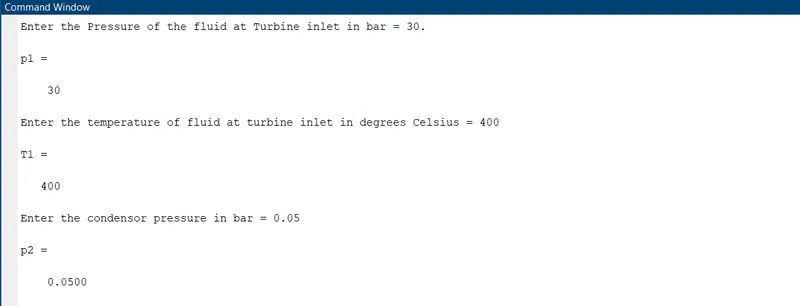
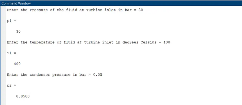
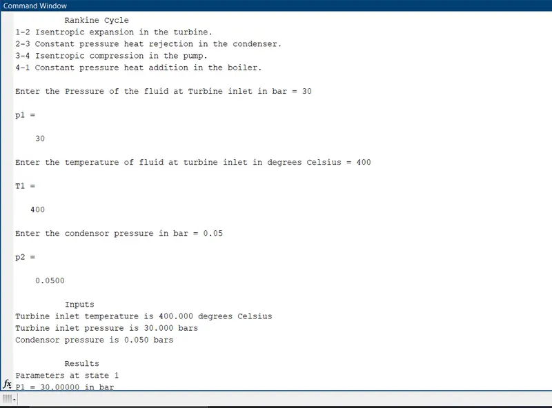
- Inputs:
- Turbine inlet temperature (T1) = 400 degrees Celsius.
- Turbine inlet pressure (P1) = 30 bars.
- Condensor pressure (P2) = 0.05 bars.
- Output:
- Temperature-Entropy diagram:
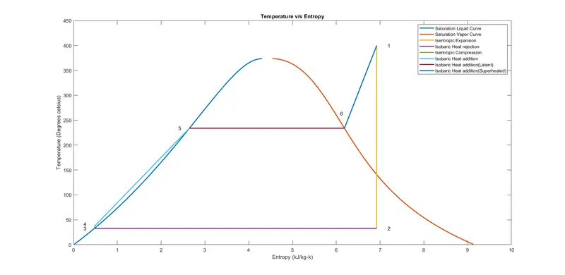
- The above graph represents the variation in the temperature and entropy of the working fluid(steam) throughout the cycle.
- Here the inlet steam to the turbine is superheated and when expanded it cool's down to the unsaturated region.
- Then the Steam coming out of the turbine is condensed in the condenser till it becomes saturated liquid at a constant temperature.
- Using the pump it's pumped to the boiler isentropically.
- In the boiler it is heated at constant pressure.
- 4-5 curve represents heating till it reaches the saturated liquid state.
- 5-6 curve represents heating till the saturated liquid becomes saturated vapor (latent heating).
- 6-1 curve represents heating the saturated vapor till it becomes superheated.
- Enthalpy-Entropy diagram:
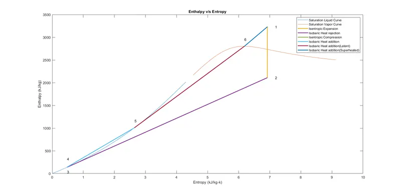
- The above graph represents the variation in the enthalpy(y-axis) and entropy(x-axis) of the working fluid(Steam) throughout the cycle.
- The saturation curves are represented in the graph.
- 1-2 and 3-4 curves represent the isentropic expansion and compression.
- 2-3 curve represents the constant pressure heat rejection.
- 4-1 curve represents the constant pressure heat addition.
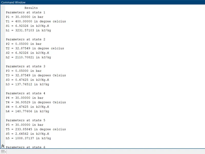
- Net work output = 1117.85188 kJ/kg.
- Back work ratio = 0.00269.
Note: The XSteam library should be in the same folder as the program file.
Conclusion:
- A program to simulate the Rankine cycle is successfully created using MATLAB as software.
- All the state points can be successfully calculated using the program.
- The XSteam library was incorporated for extraction of the state properties.
- The complete step-by-step in detail explanation of the process is documented in the report.
- The results are displayed as output for the input conditions provided and the graphs are plotted i.e. T-S( Temperature-Entropy) and H-S (Enthalpy-Entropy).
References:
- Bruce G. Miller,
7 - Clean Coal Technologies for Advanced Power Generation,
Editor(s): Bruce G. Miller,
Clean Coal Engineering Technology,
Butterworth-Heinemann,
2011,
Pages 251-300,
ISBN 9781856177108,
https://doi.org/10.1016/B978-1-85617-710-8.00007-8.
(https://www.sciencedirect.com/science/article/pii/B9781856177108000078) - Aldo Vieira da Rosa, Juan Carlos Ordóñez,
Chapter 3 - Mechanical Heat Engines,
Editor(s): Aldo Vieira da Rosa, Juan Carlos Ordóñez,
Fundamentals of Renewable Energy Processes (Fourth Edition),
Academic Press,
2022,
Pages 105-160,
ISBN 9780128160367,
https://doi.org/10.1016/B978-0-12-816036-7.00013-0.
(https://www.sciencedirect.com/science/article/pii/B9780128160367000130) -
Book by P. K. Nag