Week 5 - Genetic Algorithm
Aim: To optimize the Stalagmite function and obtain the Global maximum for the stalagmite function using the Genetic Algorithm and explain the various ways of approach with there significance.
Objective of the project:
- Specify the area of Stalagmite function.
- Code the function for the Stalagmite.
- Plot the surf for the Stalagmite output.
- Now using the Genetic Algorithm find the optimized Global maximum for the Stalagmite output.
- Here three cases are taken to obtain the Global maximum for the function output:
- Unbounded (No upper and lower bounds are defined).
- Bounded (Upper and lower bounds are defined for the GA).
- Bounded with modified Population size (Along with upper and lower bound the population size is altered).
- The results are plotted and the significance and draw backs of the case are studied.
- Stopping criteria, significance of running multiple iterations are explained.
Theory:
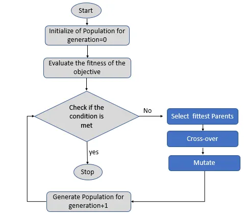
- Genetic algorithm is the optimization method which uses the Natural selection theory of Evolution.
- It may be constrained or unconstrained.
- Representation of work flow of the genetic algorithm is shown below:
- Stopping criteria:
- These are the conditions if any one of it is satisfied the Genetic algorithm stops.
- There are seven stopping criterias:
- MaxGenrations: The genetic algorithm stops when the generations reaches maximum defined/default generations.
- MaxTime: The genetic algorithm stops when it has run for the given MaxTime.
- FitnessLimit: The best point in the current populaition is taken and if the value of fintness function of the point is less than or equal to the FittnessLimit.
- MaxStallGenerations: If the average relative change in the fitness function value over the MaxStallGenerations is less than Function tolerance the then the algorithm stops.
- MaxStallTime: During the Max StallTime (in seconds) if there is no improvement in the objective function then algorithm stops.
- FunctionTolerance: Until the average relative change in the fitness function valueover MaxStallGenerations is less than the function tolerance the solution/algorithm runs.
- ConstraintTolerance: It is used to determine the feasibility with respect to the non linear constraints.
- Genetic algorithm syntax:
- [x, fval] = ga(fun, nvars, A ,b, Aeq, beq, Lb, Ub, nonlcon, IntCon, options)
- The above syntax represents the Genetic algorithum syntax.
- fun - represents the function to be optimized.
- nvars - represents the number of variables of the function to be optimized.
- A & b - Linear inequality constraints (A = Real Matrix, b = Real vector).
- Lb & Ub - Linear equality constraints (A = Real Matrix, b = Real vector).
- nonlcon - Ninlinear constraints.
- options - Optimization options.
- Intcon - Indices Integers variables.
- Significance of running multiple iterations: The cases are run for multiple time to ensure that there are no multiple outputs at a particular time for the optimized results indicating the in improper/unacceptable output.
Content of the body:
- Code Explanation:
- Start the code with clearing all the garbage values, closing all the grapgs windows and clearing the command window using the clear all, close all and clc respectively.
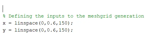
- Defining the inputs for mesh grid:
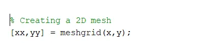
- Creating the 2D grid with x and y values using the "meshgrid" command:
- Now calling the stalagmite function with 2D matrix grid as a input.
- Creating the two for loops so to traverse through each row providing the present values as an input to the stalagmite function.
- The x and y values at the particular grid points are taken as the inputs for the stalagmite function.
- The x and y values are assigned to the variable 'input vector( )'.
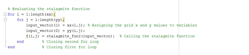
- Here the x and y values are packed for the stalagmite function and unpacked and used in the stalagmite function (By assigning the xx and yy as input_vector).
- Stalagmite function gives the z values for the x and y axis values with the formula given.
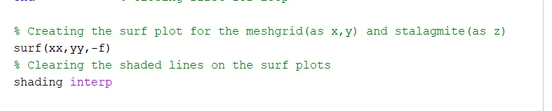
- Creating the surface plot for the output from the stalagmite function using the surf command and to remove the lines the shading interp command is used:
- Now there are three cases to understand the GA working and alteration according to the requirements:
- Case-1 Unbounded:
- Here there are no upper and lower bounds as it leads in randomly selecting the values which may even be outside the region under study.
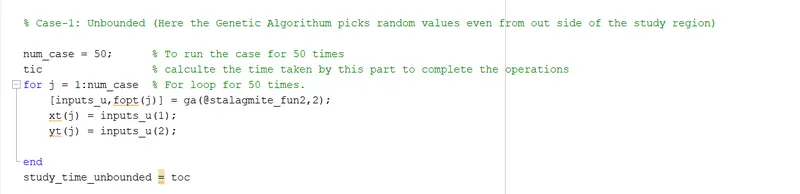
- The num_case represents the number of time the for loop is repeated.
- It is done to ensure that there is higher probability of getting the desired results with lower error/deviation.
- Here a for loop is used to repeat the case.
- The inputs_u in the LHS of the command represents the x and y values of the optimized output.
- The fopt_u represents the optimum values from the stalagmite function.
- The x and y co-ordinates for the 50 number of cases are stored in the xt( ) and yt( ) variables used to plot the graphs.
- There are two variables in the stalagmite function so the ga has 2 in its syntax.
- Tic before the loop and toc after the loop are added to output the time taken by the part of the program to execute.
- Using the ga( ) the genetic algorithm is called for the stalagmite function with two variables.
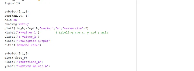
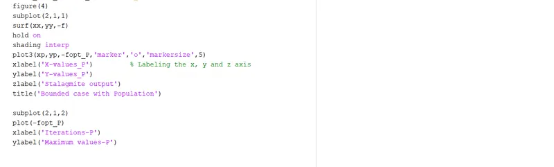
- Now the output are plotted using the plot3( ) and plot commands with the subplot option so to arrange the plots in single figure with m/n rows(2/1).
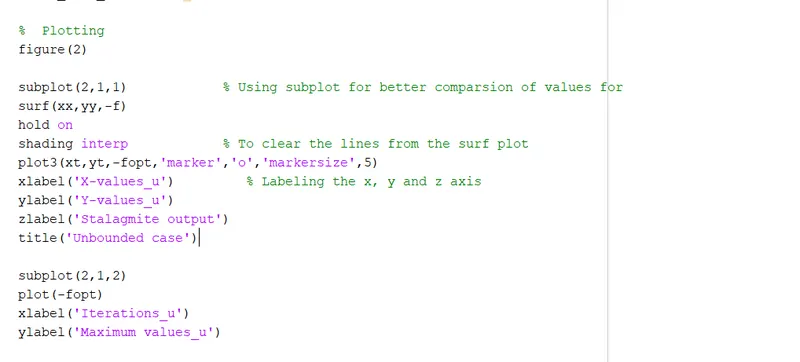
- The first plot represents the xt along x-axis, yt along y-axis and optimized maximized output along z-axis.
- The second plot represents the optimized values along y-axis for the 50 number of iteration along x-axis.
- The respective labelling are made.
- The marker in the plot syntax is used to add the markers at the value options.
- Markersize defines the size of the marker i.e. 5.
- xlabel, ylabel and zlabel are for labelling the respective axis.
- tilte command is used for adding the title to the plot.
- The outline body of this code remains same while the syntax of the GA has some additional inputs.
- Case-2 Bounded:
- In this case the lower and upper bounds are defined so as to define the selection workspace which compared to previous one was a random selection.
- Here we can consider the case to be more practically confined to the area under research.
- This is done to narrow the initial selection area.
- This case is very similar to the case-1 but only differs in the area of selecting the random population.
- This code is also much similar to the case-1 but differs in the syntax extension of the genetic algorithm command function, as here the upper and lower bounds are also defined.
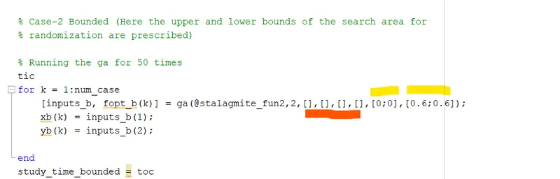
- The yellow marking represents the syntax of Genetic algorithm defining the lower and upper bounds in format ([lower x;lower y], [Upper x; Upper y]).
- Here as we know the x and y-values start from zero and end at 0.6 so the upper and lower bounds are defined in a way to fully cover the area of the meshgrid generated.
- Here the coding is similar as that of the case-1 but differ only in the above defined terms.
- Plotting:
- Case-3 Bounded with modified population size:
- Here along defining the lower and upper bounds the size of the random selection of the population is redefined.
- This is done so to have more number of initial samples which will inturn results in having the higher chance of getting the more accurate optimized output.
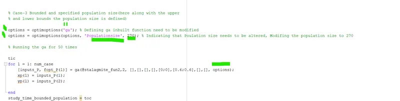
- Here the options command is used in altering the inbuilt default settings of the genetic algorithm function.
- First the options command is used to define the Function which is being altered, here as genetic algorithm is being altered adding it to the options syntax.
- Second time the option command is used to define the parameter that need to changed in predefined function, here the population size needs to be altered with new value as 270 which is defined in the second part of second option command.
- Now the changed settings needs to be used in the GA so to specify in which the case it should be used the options command is used in the syntax of the GA representing that this case needs to consider the altered default settings and no the other, this is highlighted in the code below.
- Plotting:
- Case-1 Unbounded:
- Start the code with clearing all the garbage values, closing all the grapgs windows and clearing the command window using the clear all, close all and clc respectively.
- The output of the stalagmite function gives you most of the values/peaks in the positive side, as the genetic algorithm optimizes to only minimum values we must inverse the graph (in z-axis) and find the optimum value and then inverse (multiply by negative) this value to get the global maxima of the stalagmite function, this is the reason that there is the negative sign with optimized values during the plotting of the global maxima value.
- As we calculate the global minima in the negative z-axis inverting output will result in global maxima value, as the stalagmite output is already inversed resulting the maximum values to be the minimum values.
- Stalagmite function:
- The stalagmite function is used to generate the inputs for the genetic algorithm:
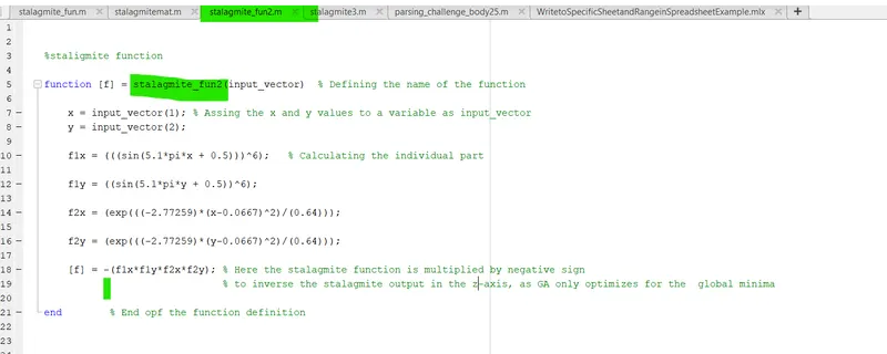
- The function command is used to create a function.
- Then and y are the inputs and are defined to the variables input_vector.
- The given equations are calculated and multiplied by negative sign to invert the stalagmite output in the z-axis, resulting in the values to turns to negative axis were maximum becomes minimum.
- The function name and the file name must be same.
- Code-Genetic Algorithm:
-
close all     % Closing all the open graphs tabs
clear all     % Clearing all the garbafge values
clc           % Clearing the command tab


% Defining the inputs to the meshgrid generation
x = linspace(0,0.6,150);
y = linspace(0,0.6,150);

% Creating a 2D mesh
[xx,yy] = meshgrid(x,y);

% Evaluating the stalagmite function
for i = 1:length(xx);
    for j = 1:length(yy);
        input_vector(1) = xx(i,j); % Assigning the grid x and y values to variables
        input_vector(2) = yy(i,j);
        f(i,j) = stalagmite_fun2(input_vector);  % Calling the stalagmite function
    end        % Closing second for loop
end            % Closing first for loop

% Actual plot output of the stalagmite function:
figure(1)
surfc(xx,yy,-f)
xlabel('x-axis')
ylabel('y-axis')
zlabel('Stalagmite output')
title('Actual')
shading interp % Clearing the shaded lines on the surf plots

% Creating the surf plot for the meshgrid(as x,y) and stalagmite(as z)

figure(2)
surfc(xx,yy,f)
xlabel('x-axis')
ylabel('y-axis')
zlabel('Stalagmite output')
title('Inverted')
% Clearing the shaded lines on the surf plots
shading interp

% Case-1: Unbounded (Here the Genetic Algorithum picks random values even from out side of the study region)

num_case = 50;      % To run the case for 50 times
tic                 % calculte the time taken by this part to complete the operations
for j = 1:num_case  % For loop for 50 times.
    [inputs_u,fopt(j)] = ga(@stalagmite_fun2,2);
    xt(j) = inputs_u(1);
    yt(j) = inputs_u(2);

end
study_time_unbounded = toc

%  Plotting
figure(3)

subplot(2,1,1)            % Using subplot for better comparsion of values for
surf(xx,yy,-f)
hold on
shading interp            % To clear the lines from the surf plot
plot3(xt,yt,-fopt,'marker','o','markersize',5)
xlabel('X-values_u')         % Labeling the x, y and z axis
ylabel('Y-values_u')
zlabel('Stalagmite output')
title('Unbounded case')

subplot(2,1,2)
plot(-fopt)
xlabel('Iterations_u')
ylabel('Maximum values_u')


% Case-2 Bounded (Here the upper and lower bounds of the search area for
% randomization are prescribed)

% Running the ga for 50 times
tic
for k = 1:num_case
    [inputs_b, fopt_b(k)] = ga(@stalagmite_fun2,2,[],[],[],[],[0;0],[0.6;0.6]); % Defining the bounds
    xb(k) = inputs_b(1);
    yb(k) = inputs_b(2);

end
study_time_bounded = toc
% Plotting
figure(4)

subplot(2,1,1)
surf(xx,yy,-f)
hold on
shading interp
plot3(xb,yb,-fopt_b,'marker','o','markersize',5)
xlabel('X-values_b')         % Labeling the x, y and z axis
ylabel('Y-values_b')
zlabel('Stalagmite output')
title('Bounded case')

subplot(2,1,2)
plot(-fopt_b)
xlabel('Iterations_b')
ylabel('Maximum values_b')


% Case-3 Bounded and specified population size(here along with the upper
% and lower bounds the population size is defined)

options = optimoptions('ga'); % Defining ga inbuilt function need to be modified
options = optimoptions(options, 'Populationsize', 270); % Indicating that Poulation size needs to be altered, Modifing the population size to 270

% Running the ga for 50 times

tic
for l = 1: num_case
    [inputs_P, fopt_P(l)] = ga(@stalagmite_fun2,2, [],[],[],[],[0;0],[0.6;0.6],[],[], options); % Calling the changed options settings for this particular case
    xp(l) = inputs_P(1);
    yp(l) = inputs_P(2);

end
study_time_bounded_population = toc
% Plotting
figure(5)
subplot(2,1,1)
surf(xx,yy,-f)
hold on
shading interp
plot3(xp,yp,-fopt_P,'marker','o','markersize',5)
xlabel('X-values_P')         % Labeling the x, y and z axis
ylabel('Y-values_P')
zlabel('Stalagmite output')
title('Bounded case with Population')

subplot(2,1,2)
plot(-fopt_P)
xlabel('Iterations-P')
ylabel('Maximum values-P')
-
- Code-Stalagmite function:
-
%staligmite function

function [f] = stalagmite_fun2(input_vector)  % Defining the name of the function

    x = input_vector(1); % Assing the input_vector values to variable as x and y (unpacking)
    y = input_vector(2);

    f1x = (((sin(5.1*pi*x + 0.5)))^6);   % Calculating the individual part

    f1y = ((sin(5.1*pi*y + 0.5))^6);

    f2x = (exp(((-2.77259)*(x-0.0667)^2)/(0.64)));

    f2y = (exp(((-2.77259)*(y-0.0667)^2)/(0.64)));

    [f] = -(f1x*f1y*f2x*f2y); % Here the stalagmite function is multiplied by negative sign
                              % to inverse the stalagmite output in the z-axis, as GA only optimizes for the  global minima

end        % End of the function definition
-

Results and discussion:
- Output of the stalagmite function (Actual and Inverted):
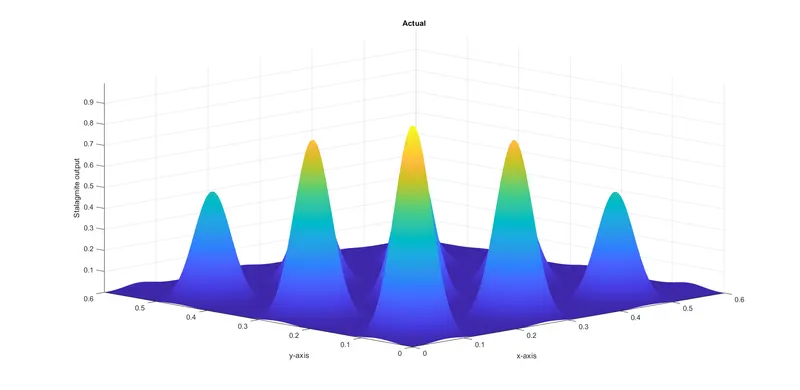
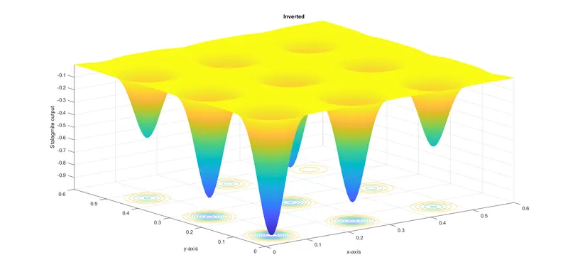
- Used to find the global minima by using the genetic algorithm.
- Case-1 Unbounded Optimized output:
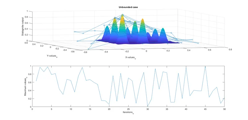
- Here in this case the algorithm choses random population without any boundaries resulting in more dispersed output.
- Here the optimized values are ranging from 0-1 which is not at all accurate.
- This case types cannot be used for this kind of function/problems.
- Here the algorithm is run for 50 times.
- Case-2 Bounded Optimized output:
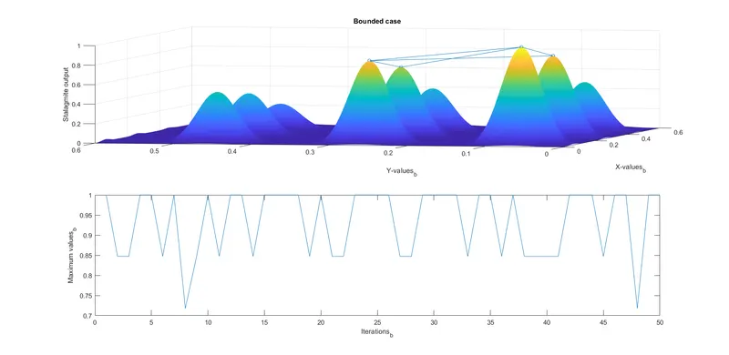
- Here the algorithm selects the population in the region defined in the upper and lower bounds.
- Here the output/optimized results are more confined and near to the optmized value compared to case-1.
- It can be seen that the optimized values are much closer to the actual maximum value (0.7 - 1) compared to case-1 (subplot - 2).
- Here the algorithm is run for 50 times.
- Case-3 Bounded with population modification Optimized output:
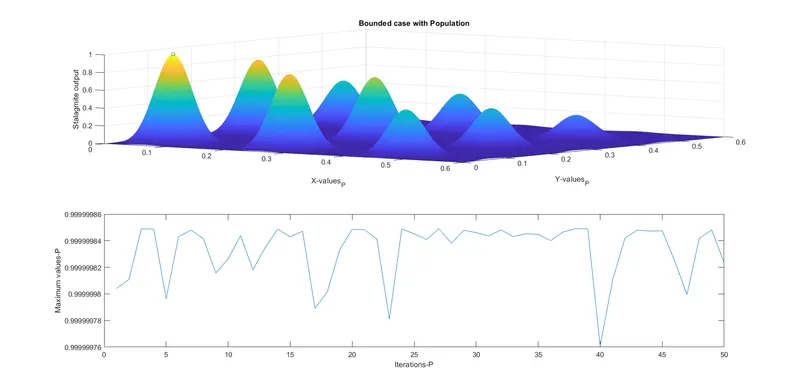
- Here algorithm selects the population in the confined region with defined population size to improve the optimized value.
- By selecting more population we have higher chance of getting to the optimized solution as the population will cover more region or points in the confined region, which will be processed to achieve the optimized results.
- Here it can be seen that the obtained optimized results are very closer to the real maximum value (0.99999976-0.99999986).
- The values are very near to the optimized values compared to any of the previous cases.
- Here the algorithm is run for 50 times.
- The algorithm is run for 50 times because to ensure there is no variation in the output optimized values.
- Stopping criteria:
- The stopping criterias for our function of Genetic algorithum are:
- Optimization terminated: maximum number of generations exceeded.
- Optimization terminated: average change in the fitness value less than options.FunctionTolerance.

- The stopping criterias for our function of Genetic algorithum are:
Conclusions:
- The program is executed successfully to obtain the optimized result for the given Stalagmite function.
- Three cases are into consideration for the study/execution:
- Case-1 Unbounded:
- Here the results obtained are completely random and out of the research space.
- Here the solution is improper as the algorithum selects the populations randomly which may even be outside the area under study.
- So this is not the proper way to use the Genertic algorithm as it does not provide any accurate optimized output.
- Case-2 Bounded:
- Here the results are significantly improved as compared to the unbounded case beacause the upper and lower bounds are defined so the population selected is in the area under study which enhances the chances of getting the optimized output too the function.
- But this is also not much efficient way to optimize the function even though it is much closer to the optimized values compared to the case-1.
- Case-3 Boundded with modified population size:
- Here the results are significantly accurate with 0.000014% Error.
- Here we get the Global maxima of 0.99999986.
- As the case-3 is giving the most accurate result it may be concluded that, to obtain the more accurate solution we must have higher population and the bounds depecting the boundaries of the area under study/interest must be defined properly.
- Also defining more boundary constraints is helpful in many of the cases.