Week 2 - Flow over a Cylinder.
Aim: To simulate the flow over a cylinder and to find the effect of Reynolds number on the co-efficient of drag and to find the Strouhal Number for the specified parameters.
Objective:
- Design the geometry as per the given conditions.
- Mesh the geomerty with the appropriate quality criteria.
- Setup the physical and boundary conditions for the flow simulation.
- Calculate the Strouhal Number for the Reynolds Number 100 with the transient state solver.
- Run the steady state simulation for varying Reynolds Number (By varying the velocity of the flow).
- Study the effect of Reynolds number on the Drag co-efficient.
Theory:
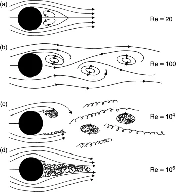
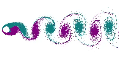
- Karman vortex street is phenomenon caused by the vortex shedding were the swirling vertices are formed from the surfaces of the blunt bodies in the wake regions.
- The Karman vortex street starts to occur at the Reynolds Number of 200 till `10^5`.
- It causes unsteady flow seperating around the blunt objects.
- Flow seperation:
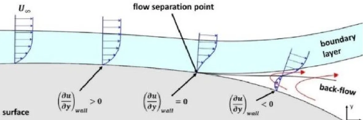
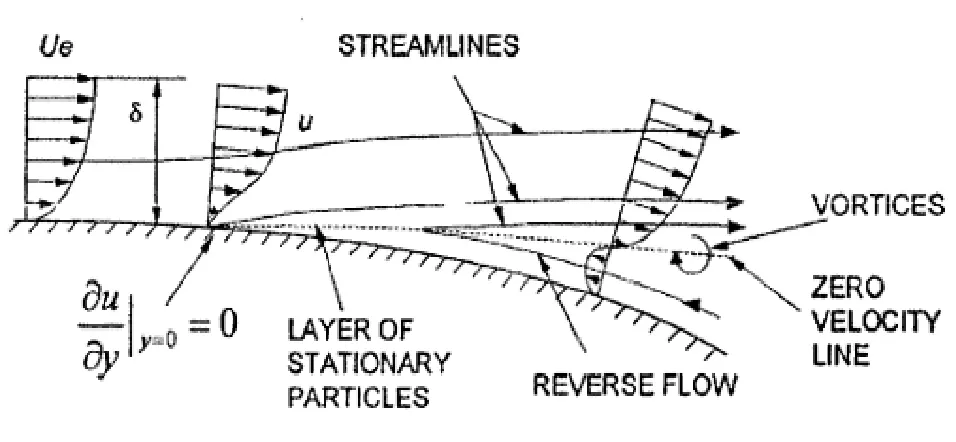
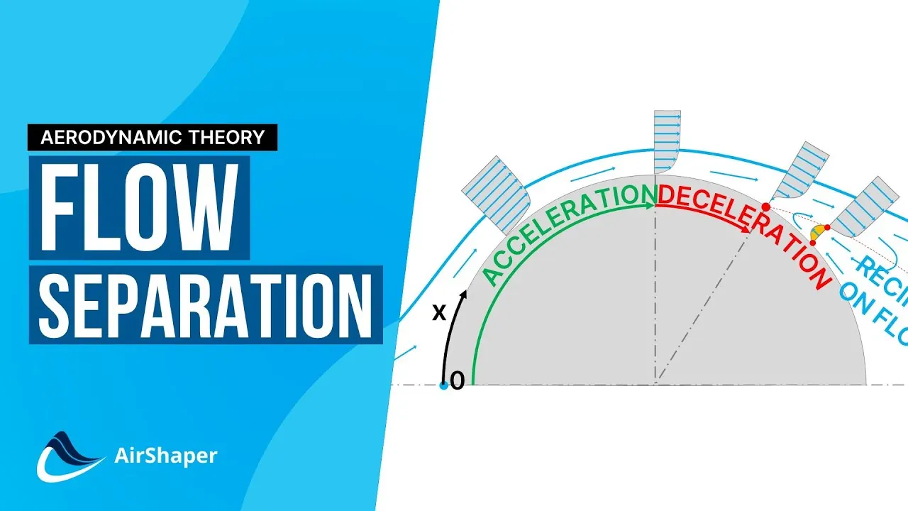
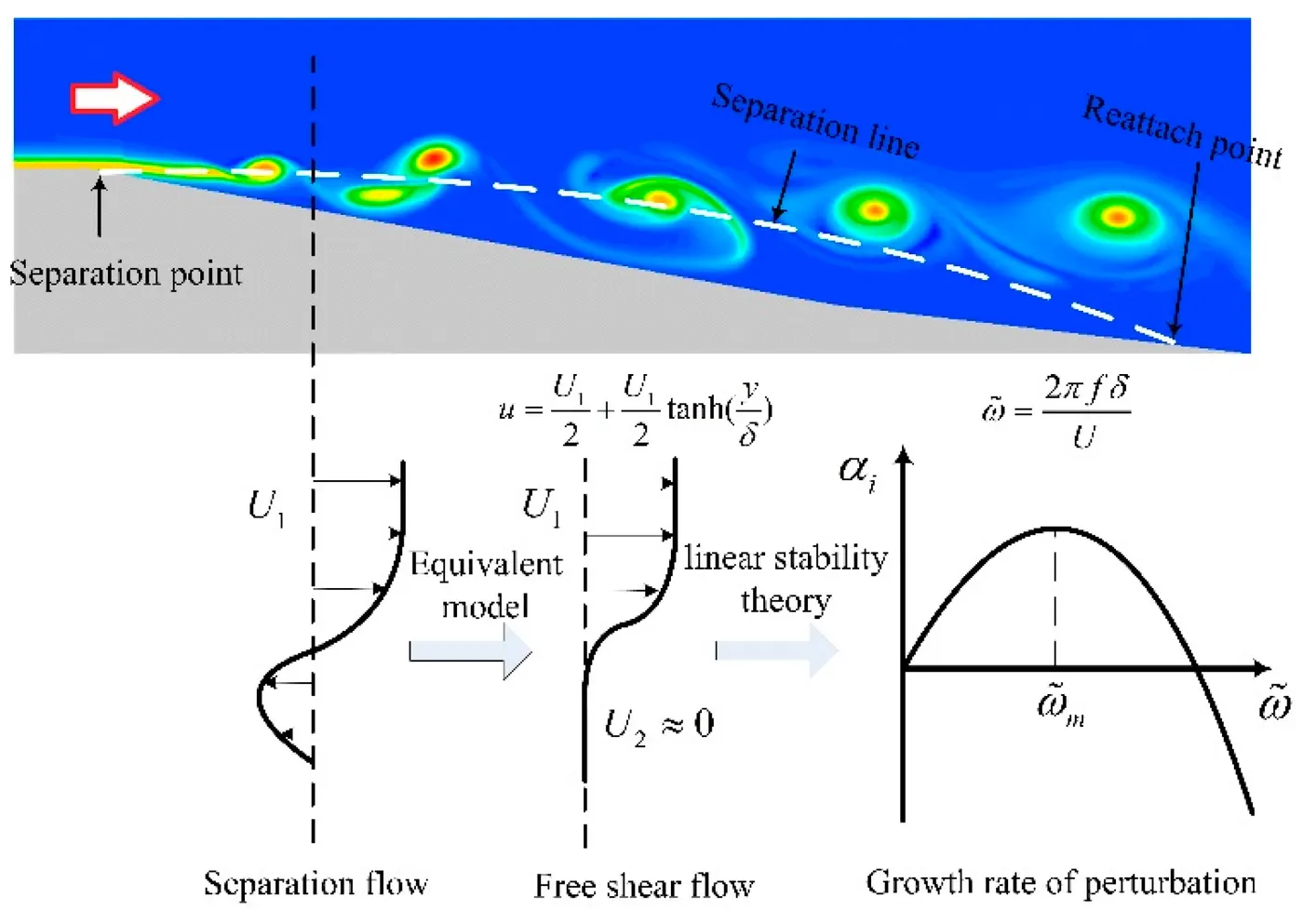
- The point at which the flow seperates from the body is called point of seperation.
- At this point the boundary of fluid flowing detaches from the body causing the backflow in the below region as shown above.
- This exertes the force on the bodies perpendicular to the flow (Cylinder) which reverses the direction every time the vortex is shed.
- This may some times be helpful but majority of times causes concerns over the Resonance frequency of the structure under study.
- For the external flows the critical Reynolds Number is 500000 (i.e. beyond which the flow becomes turbulent).
- Co-efficent of drag (cd): A dimensionless quantity which is used for measuring the drag or resistance on an object due surrounding fluid medium.
- Co-efficient of lift (cl): It is dimension less quantity which is used to relate the lift generated by a body due to density, velocity of the fluid and area of contact known as frontal area.
- Drag force(D): It is the opposition/resistance on the body due to surrounding fluid, measured in Newtons(N).
- Drag force = `1/2rho *v^2 *cd * A`
- A = fromtal area.
- v = velocity.
- `rho` = density of the fluid.
- Lift force (L): A fluid flowing. around the body experience a force one part of it is lift force which is acting in the perpendicular direction of the flow.
- Lift force = `1/2*rho*cl*v^2*A`
Content of the body:
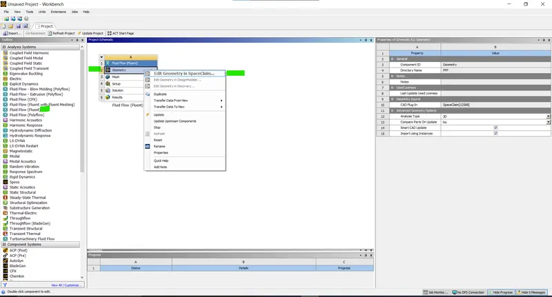
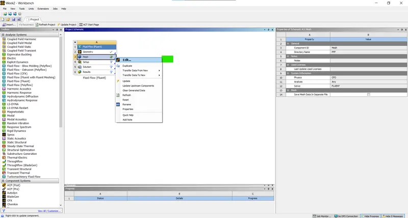
- Opening the Ansys Workbench with Ansys Fluent setup (Fluid Flow-Fluent):
- Select the spaceclaim design module for designing the geometry:
- Now design the geometry as per the given criteria:
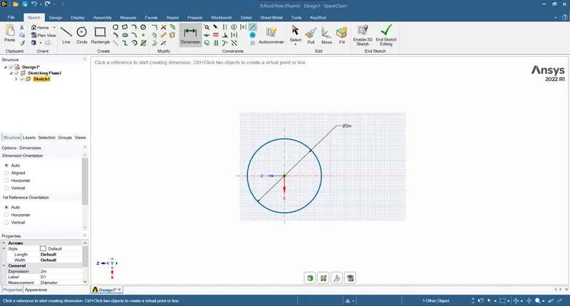
- Selec the XZ-plane:
- Circle of 2 meter diameter - 2D:
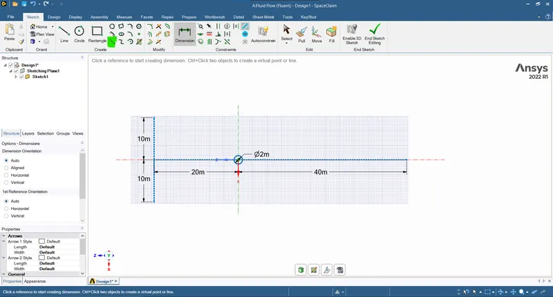
- Using the construction lines option from the tool bar draw the lines as per the given dimensions of the area around the cylinder:
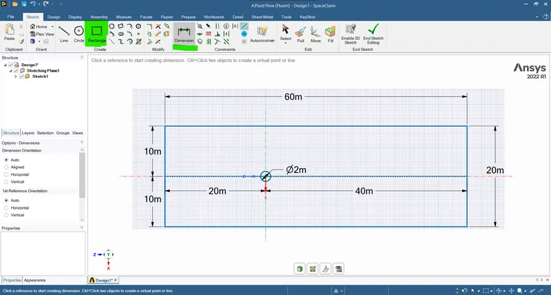
- Now use the rectangle create tool to create the rectangle using the two edges of the front construction line:
- Now using the pull command on the drawn model:
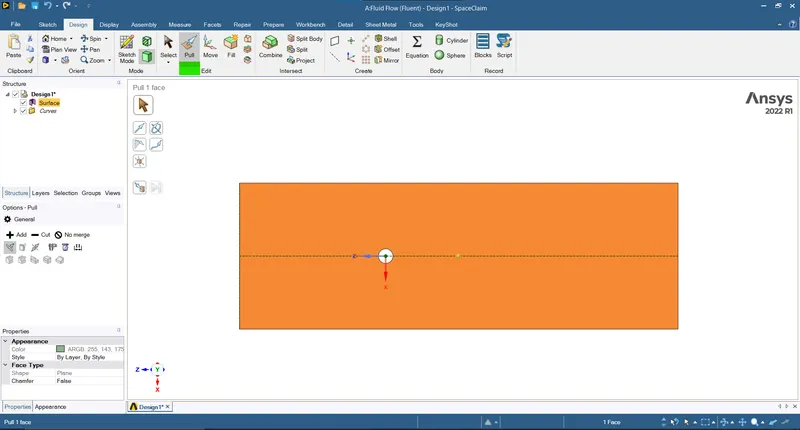
- Now the rectangular selection has changed to the surface.
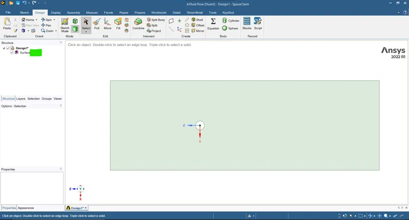
- Delete the construction lines.
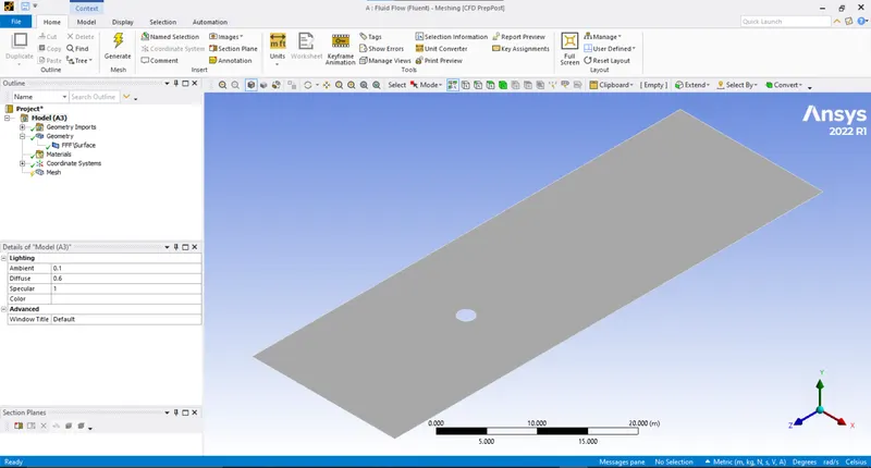
- Now the geometry design is complete.
- Exit the spaceclaim.
- Meshing:
- Open the mesh:
- Click on the generate mesh option in the mesh tool:
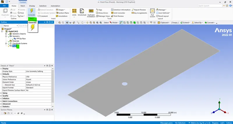
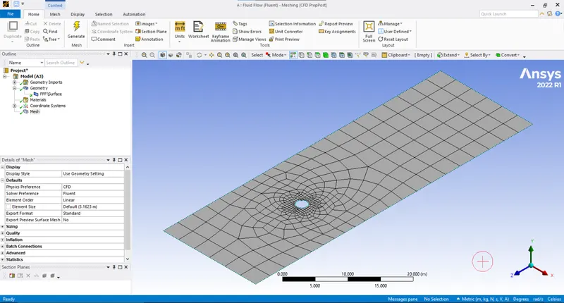
- Since the mesh is very coarse and mostly quadrilateral in elements we need to refine the mesh:
- Firstly changing the quad elements to triangular elements:
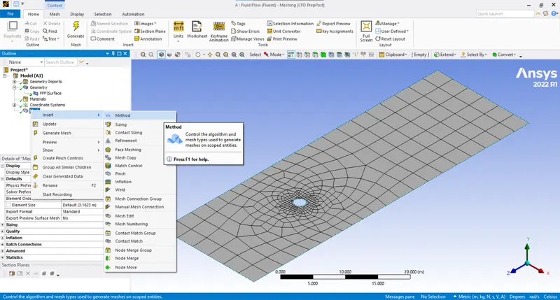
- A automatic method is used to define the tria dominent mesh (Mesh > Insert > Method > Ok):
- Now select the geometry and hit apply in the body tab:
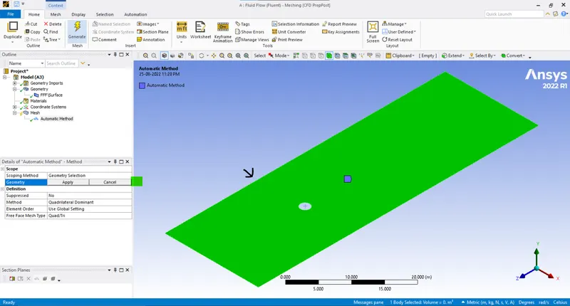
- Now change the element type to tria:
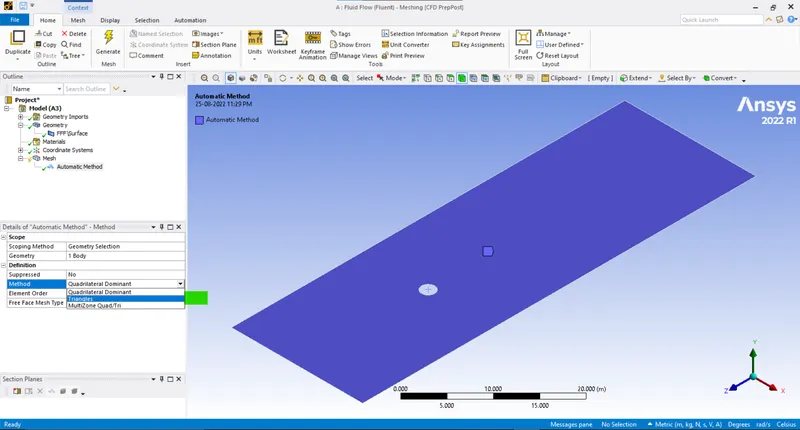
- Now the mesh is having only tria elements now the mesh size and refinement near the cylinder area need to be done:
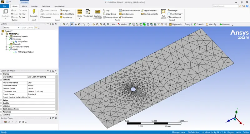
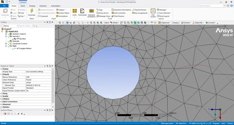
- Refining the cylinder circumference by edge sizing:
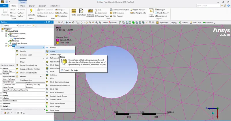
- Selecting the edge to which needs refinement:
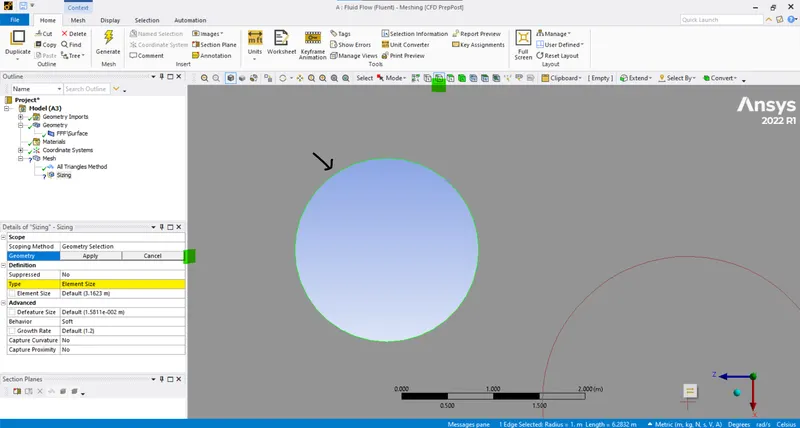
- Selecting the 'Type' to Number of Elements:
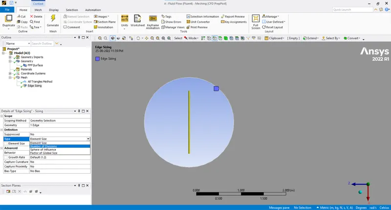
- Setting the elements numbers to 36.
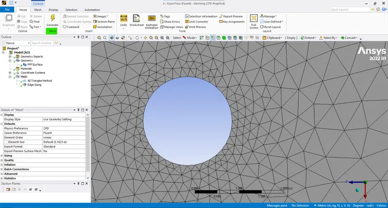
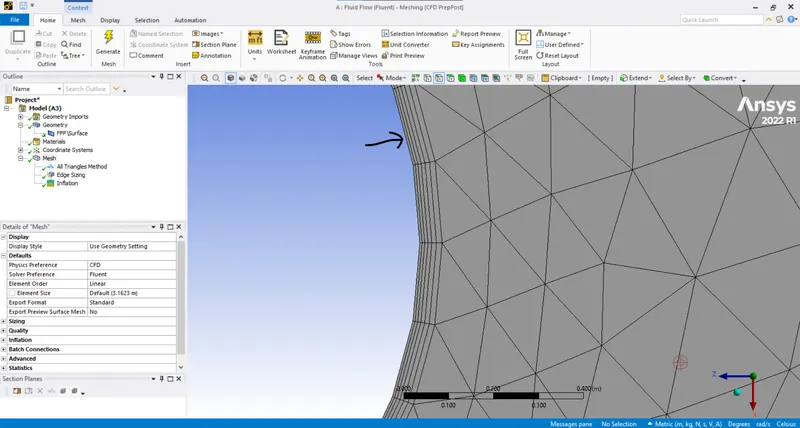
- Adding the refinement near the cylinder wall using the Inlation layers (Mesh > Insert > Inflation layers > Ok):
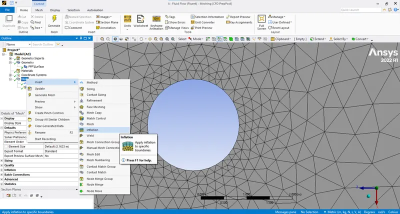
- Selecting the geometry:
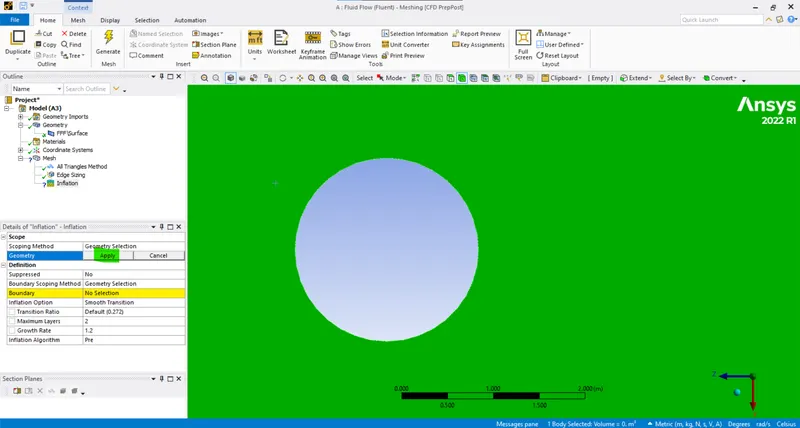
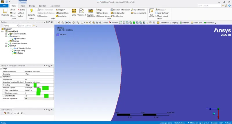
- Selecting the boundaries and define the inflation option type to First layer thickness with growth rate of 20% for each layer with initial layer of 5 mm and updating the mesh:
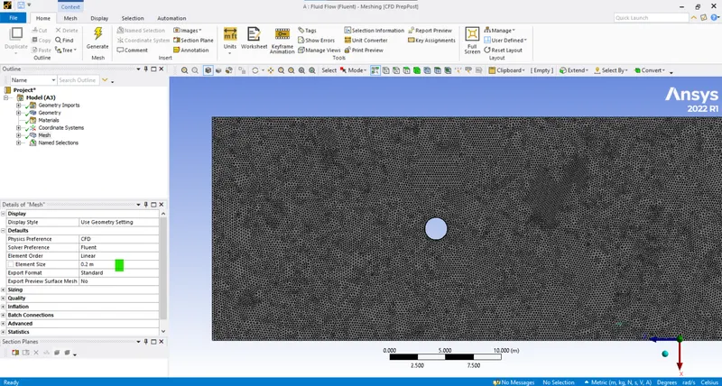
- Refining the mesh elements size (0.2m):
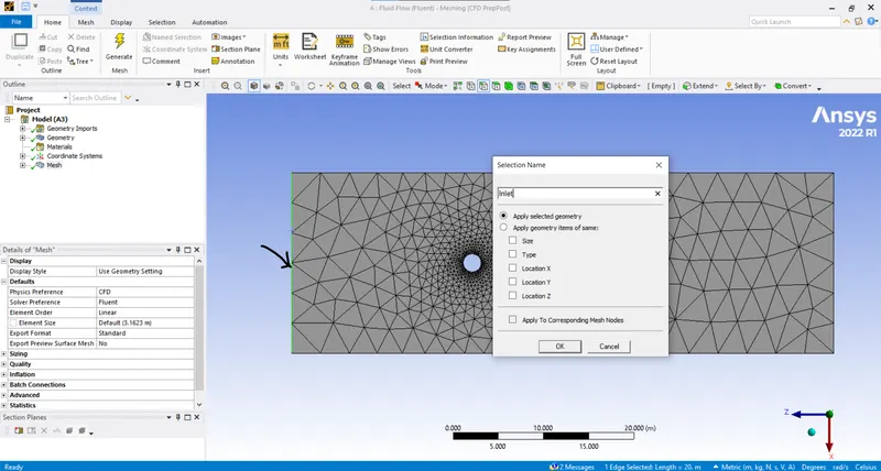
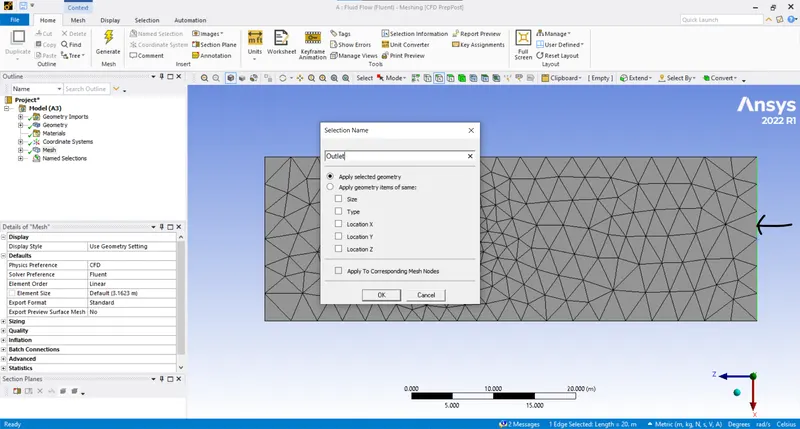
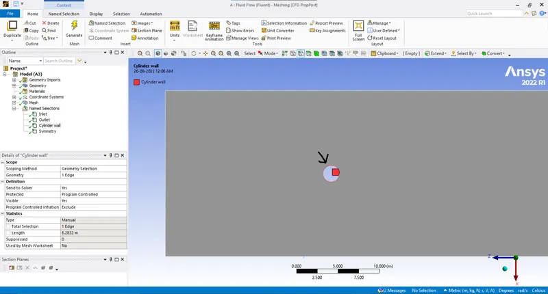
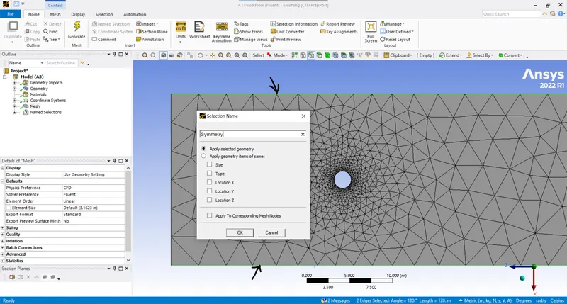
- Naming the sections(Edge selection > select th edge > Create name selection):
- Inlet:
- Outlet:
- Cylinder wall:
- Symmetry:
- Open the mesh:
- Setup up the Physics and the boundary conditions:
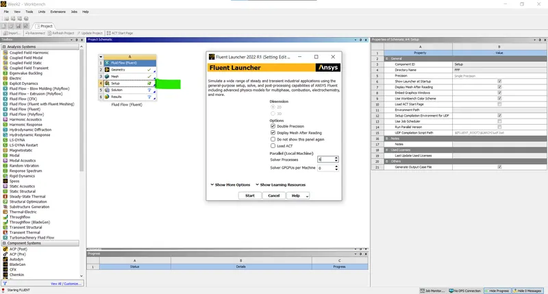
- Open the setup:
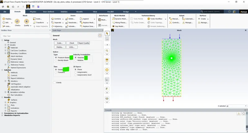
- Setting the conditions as Pressure based, Velocity formation absolute and the time as steady state:
- No need to activate the Energy model as we are not concerned with the temperature but only the flow over the cylinder.
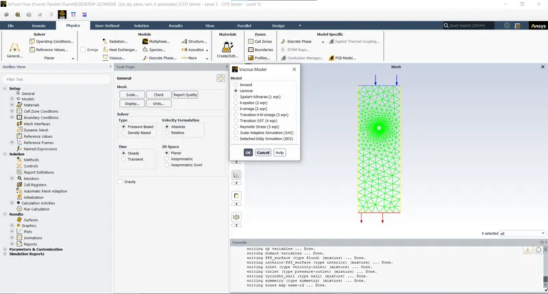
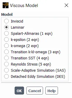
- Selecting the viscous model as laminar as for now our reynolds number will be low:
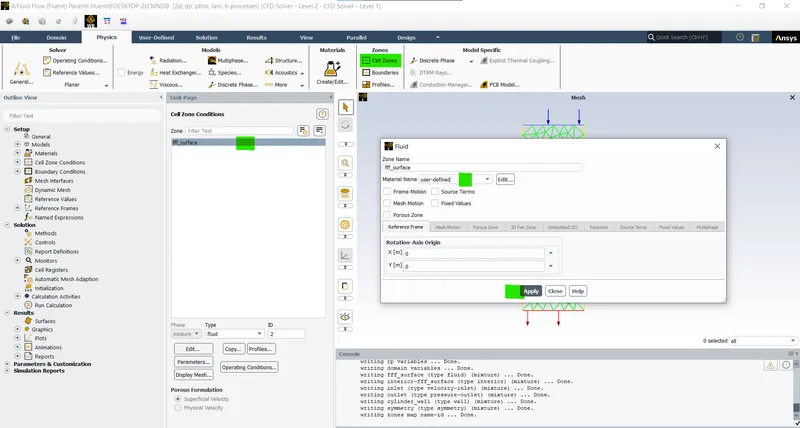
- Creating the fluid with the defined properties:
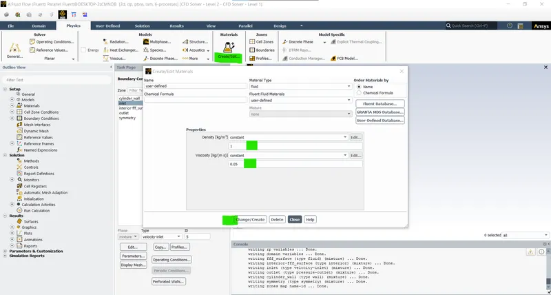
- Density = 1 kg/m^3.
- Viscosity = 0.05 kg/(m s).
- Defining the surface materials (Cell zones > Select the surface > Edit > select the material > Ok):
- Finding the velocity:
- Reynolds Number = `(Density * Velocity * Diameter)/(Viscosity)`
- Density = 1 `(kg)/m^3`
- Diameter = 2m.
- Viscosity = 0.02 `(kg)/(m*s`
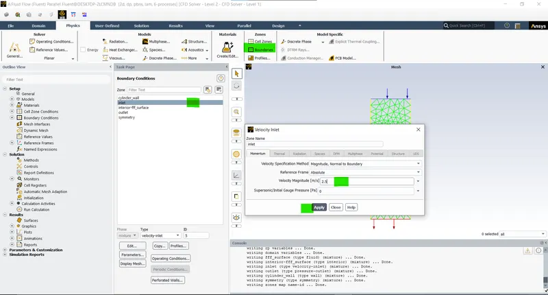
- Velocity = 2.5 m/s.
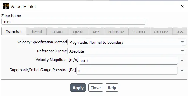
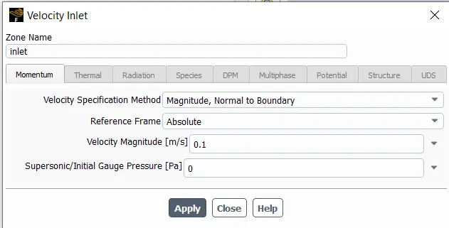
- Defining the Inlet (Boundary conditions > Inlet > Define Inlet as velocity inlet > define the velocity magnitude > Apply):
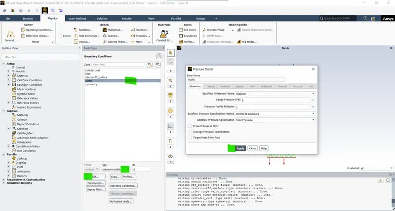
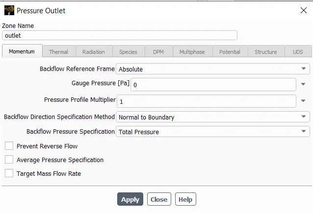
- Defining the outlet as the velocity outlet:
- Open the setup:
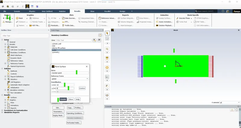
- Now to observe the vortex phenomenon by the variation of the velocity we are going to add a point (10 m from the centre of the cylinder) (Resuts > Create > Point > Set the distance from the co-ordinate > Ok):
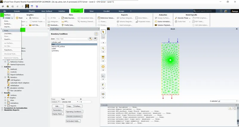
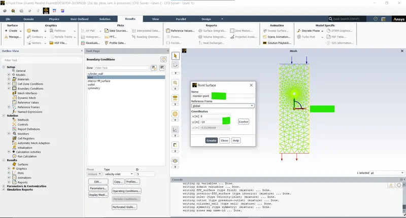
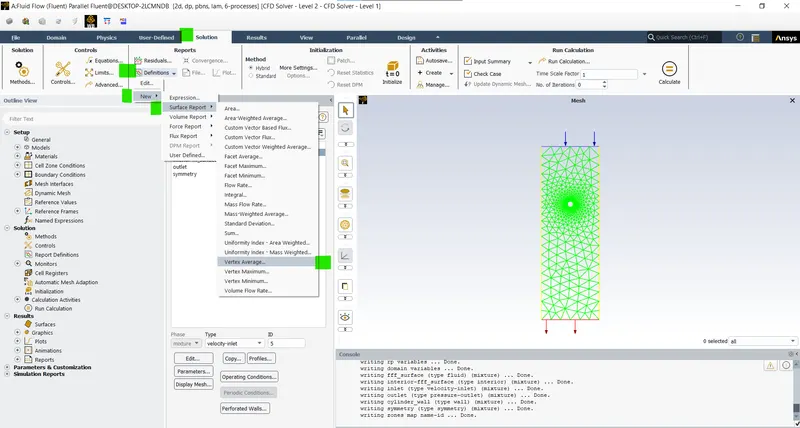
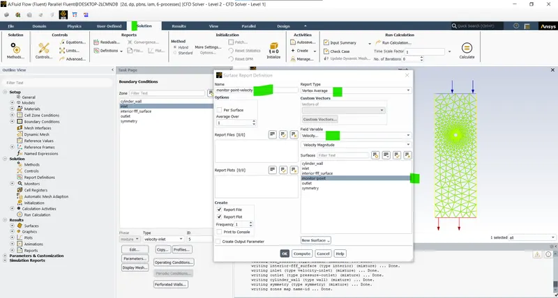
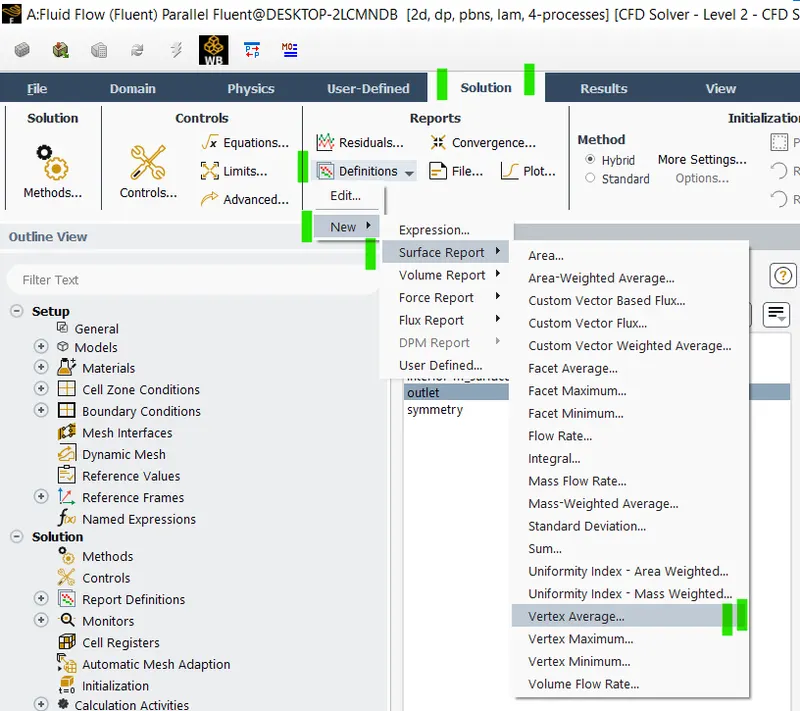
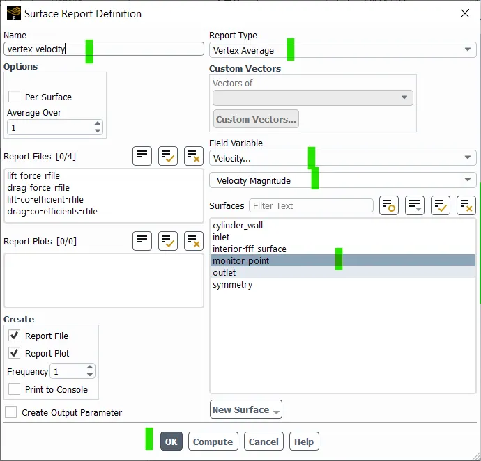
- Now defining the surface reports of Vortex:
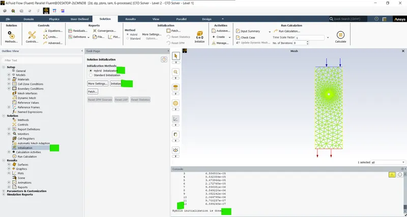
- Now initialize the system with Hybrid Initialization:
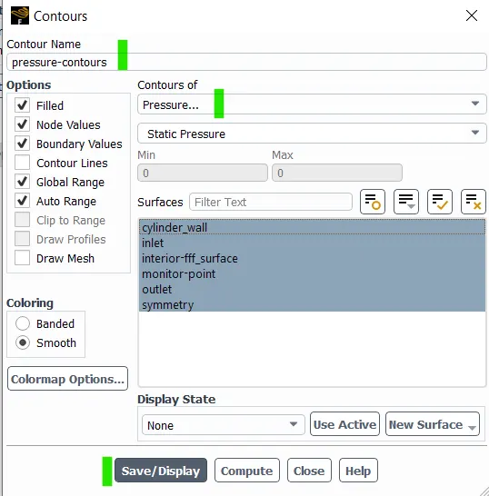
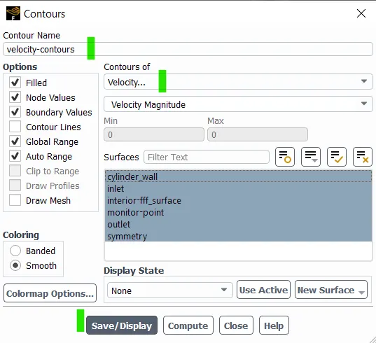
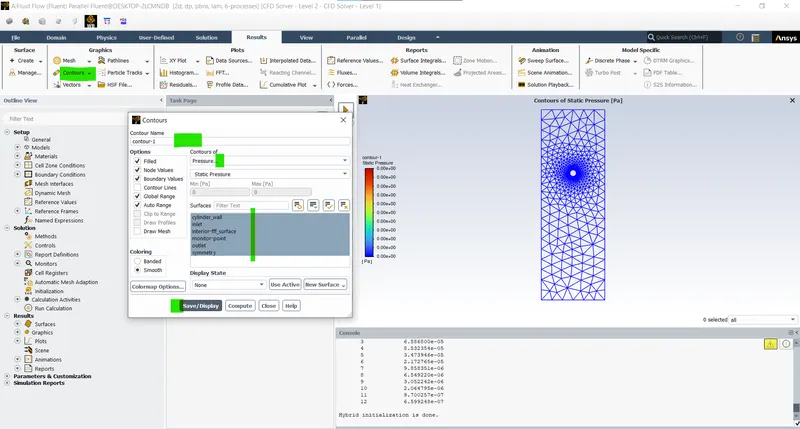
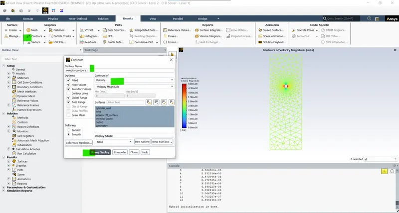
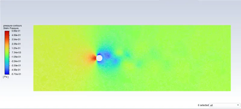
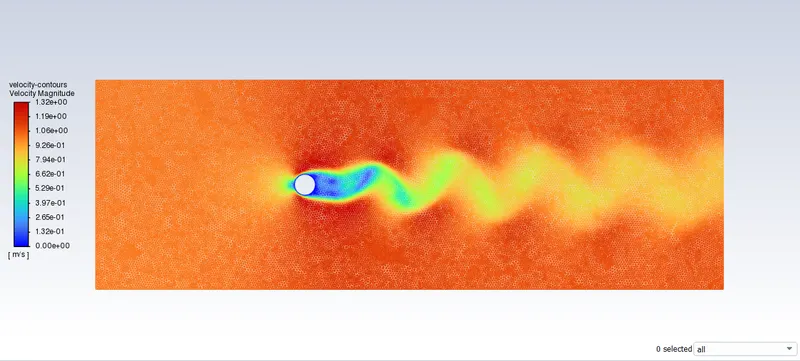
- To observe the changes in velocity and pressure during the vortex street we can add contours of pressure and velocity (Results > Pessure/Velocity > Select the regions > save and display):
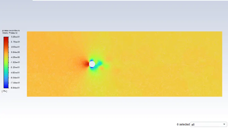
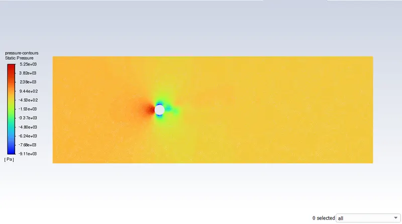
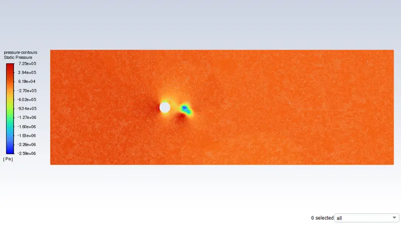
- Pressure contour:
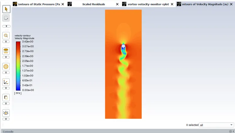
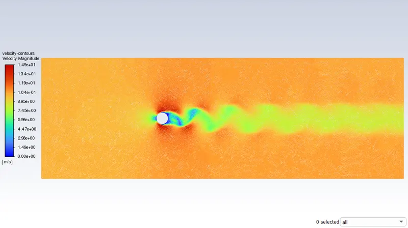
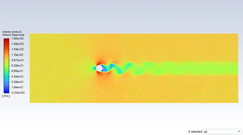
- Velocity contour:
- Pressure contour:
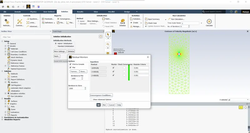
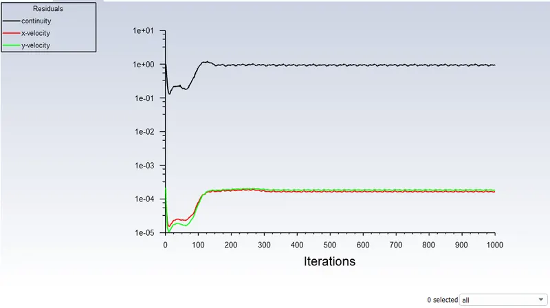
- Deselecting the convergence criterias as to reun the simulation for desired amount of time and check the convergence of a physical quantity such as velocity instead to observe the surface flow phenomenon:
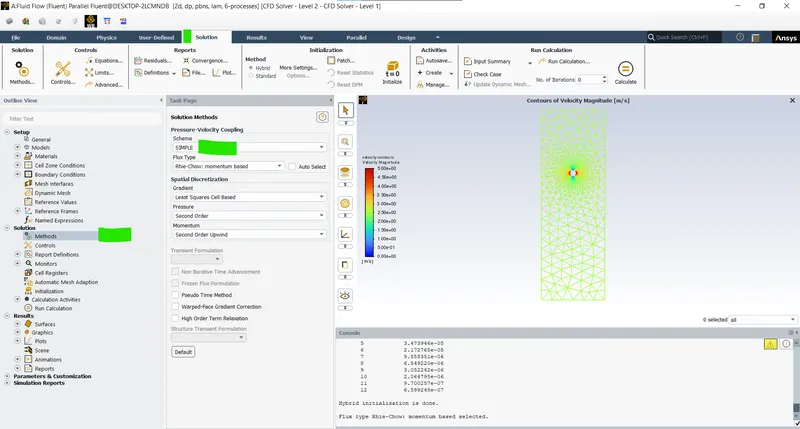
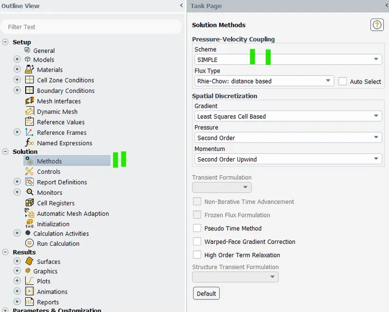
- Now defining the solver solution method:
- Here the SIMPLE method is used:
- Here the SIMPLE method is used:
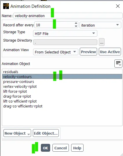
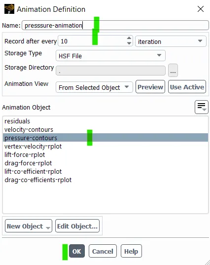
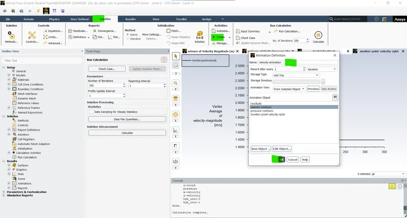
- Creating a animation of velocity (Solution > Create > animation > Select the countours > Ok):
- Now the simulation is run on th steady state time:
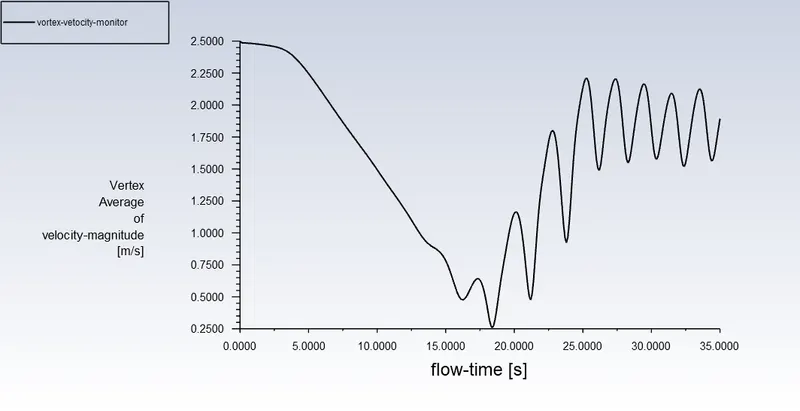
- But to calculate the Strouhal Number at Re= 100 we need to have the time period of the oscilation so switching to the transient state calculation:
- Transient state solver (Re =100):
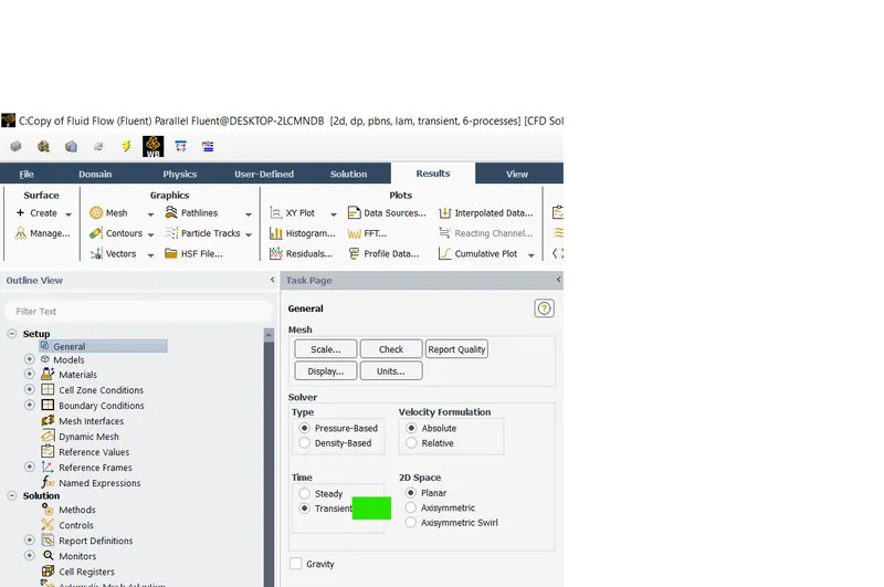
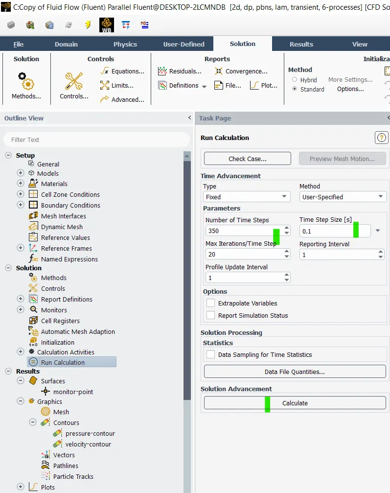
- Running the simulation for 350 number of steps with 0.1 second as time step:
- Plots after solving:
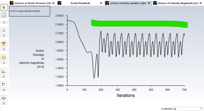
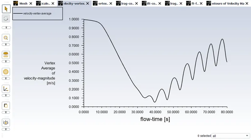
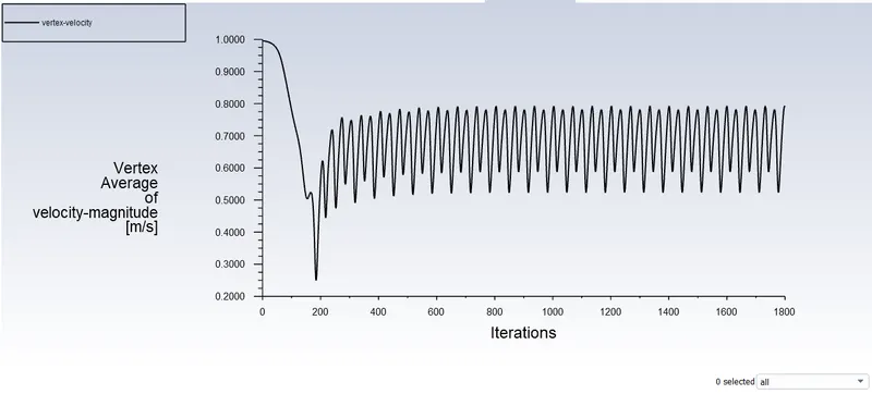
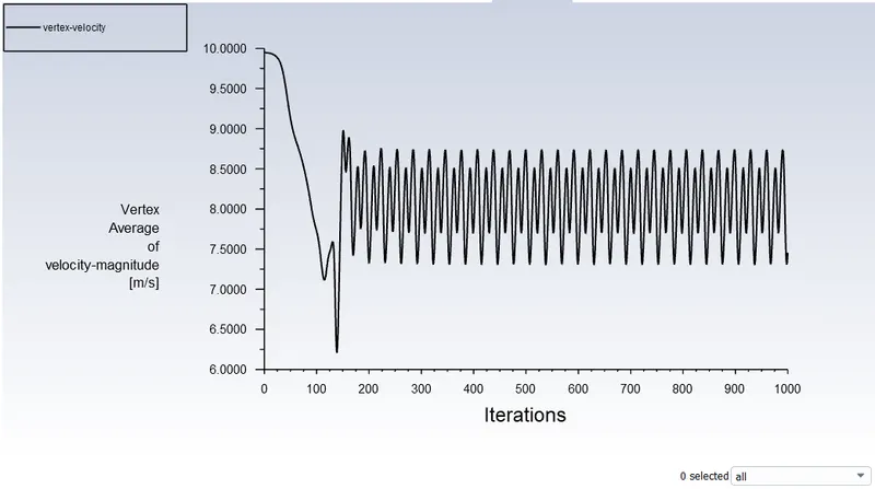
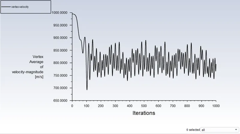
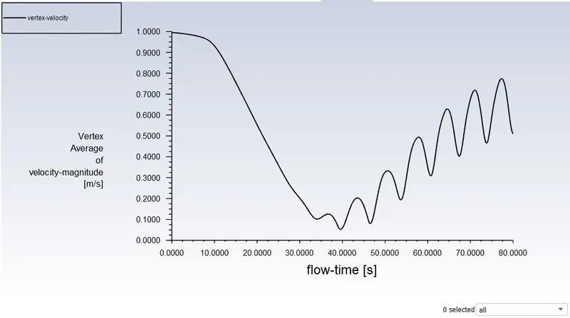
- Vertex average of velocity magnitude:
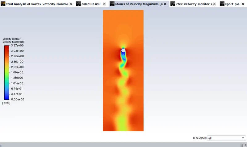
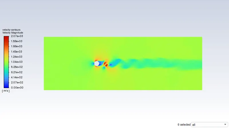
- Velocity contours:
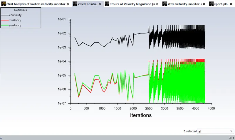
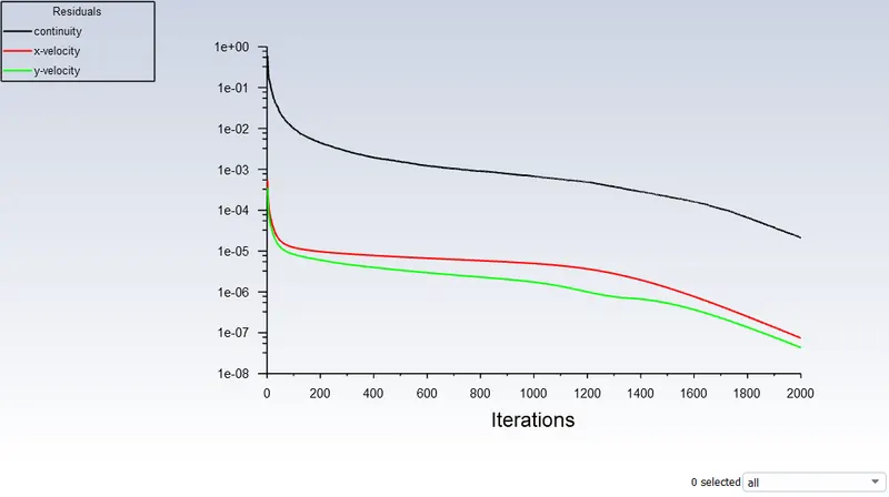
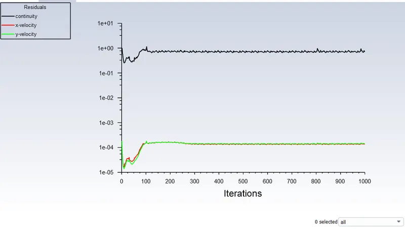
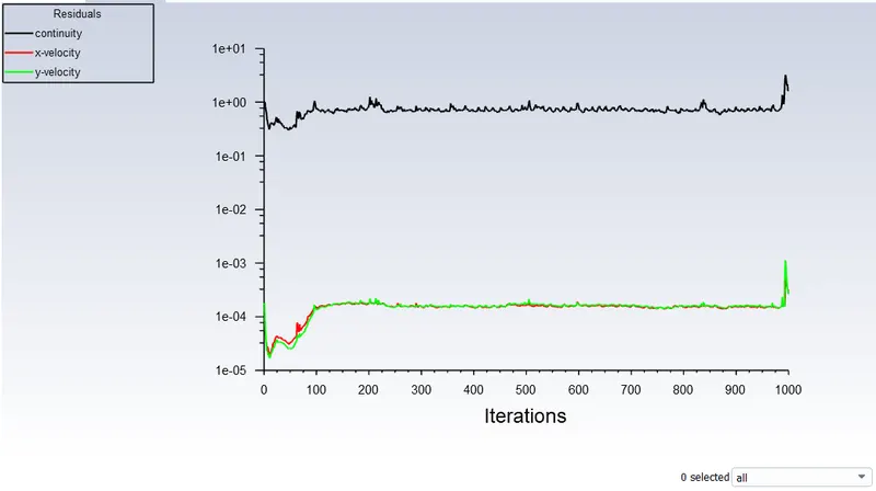
- Residuals:
- Steady state solver at Re = 10:
- All the steps are similar after selecting the steay state solver but the Reynolds number needs to be varied by varying the Velocity of the fluid.
- Defining the velocity for Reynolds number = 10:
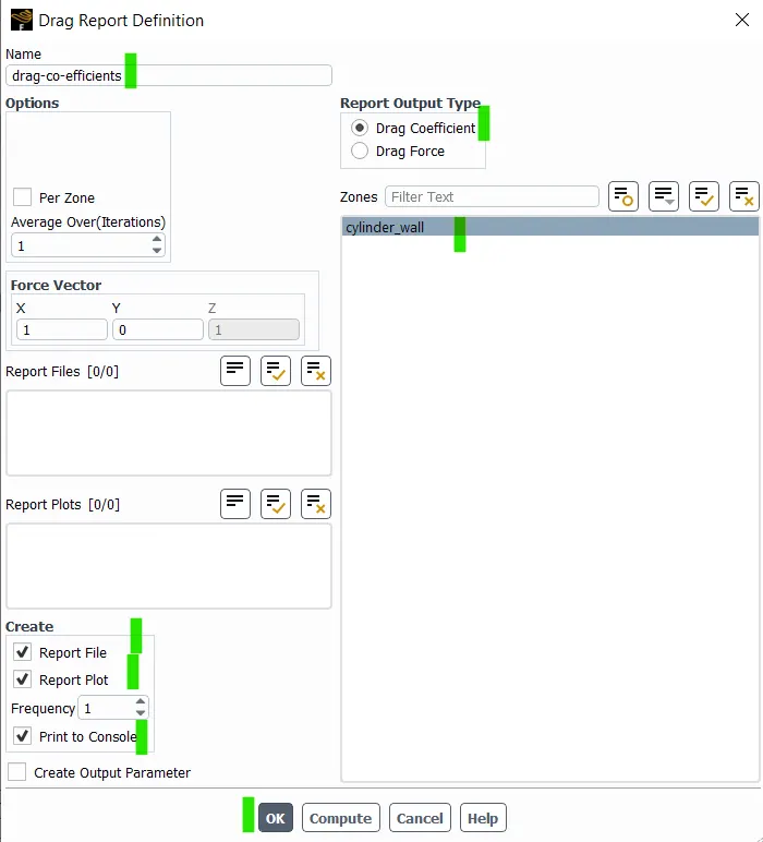
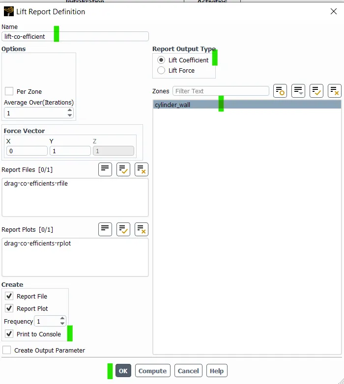
- Defining the Lift and Drag co-efficient report plot and rfile:
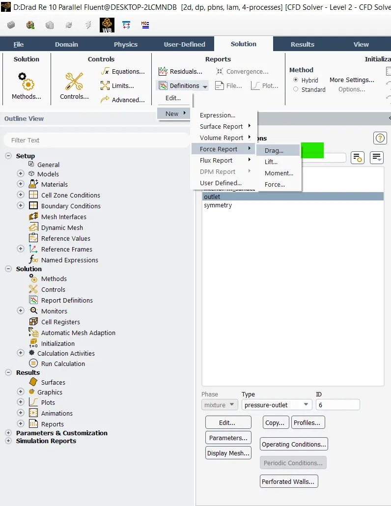
- Drag co-efficients:
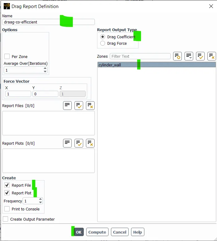
- Lift co-efficients:
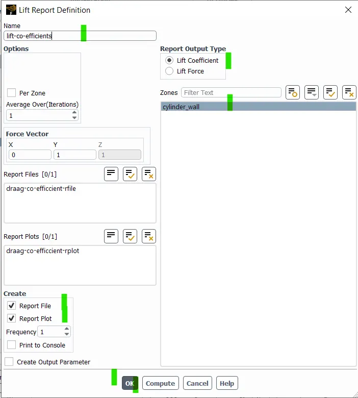
- Re - 100 Transient state solver:
- Here the conditions vary as a function of time.
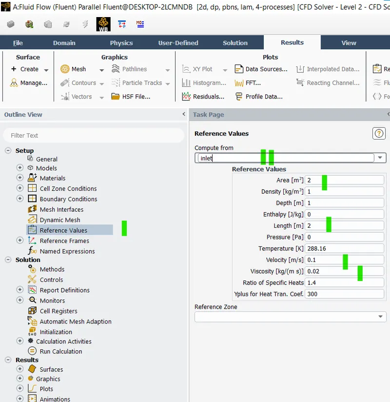
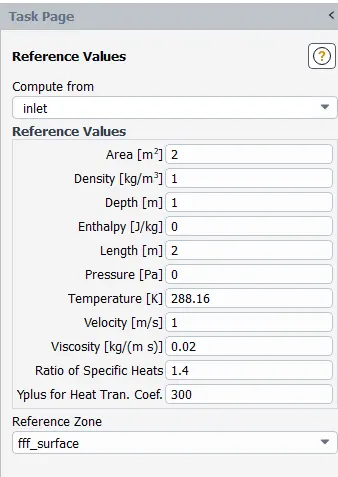
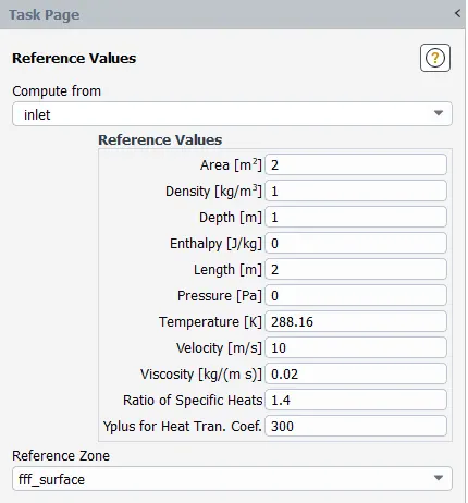
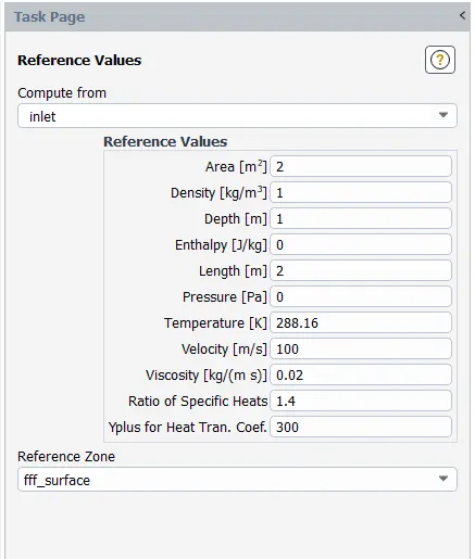
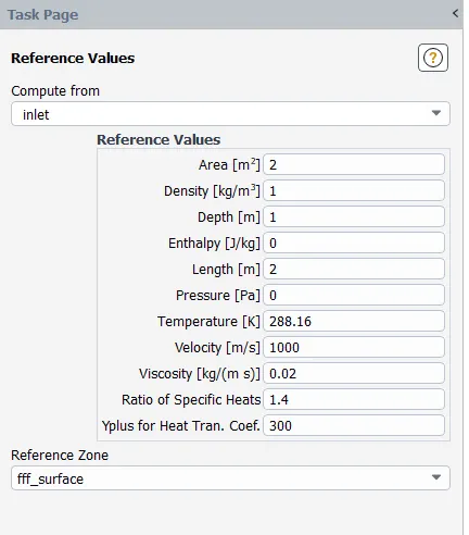
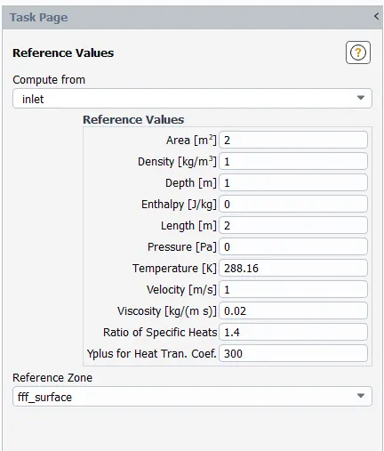
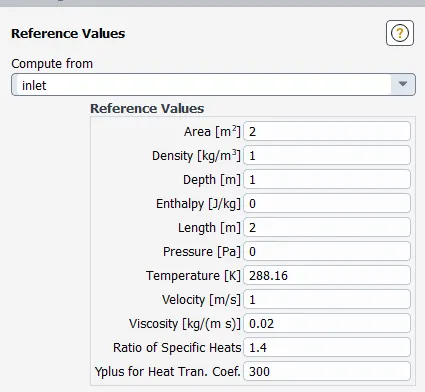
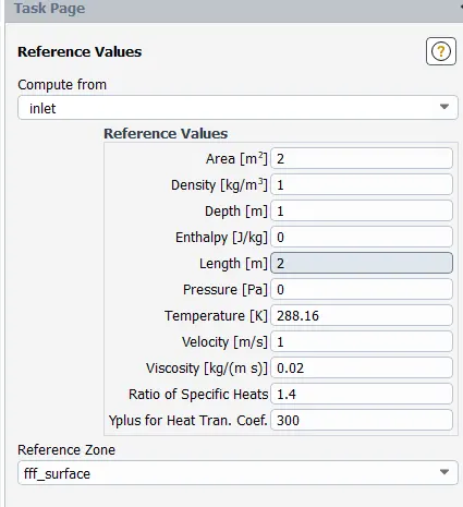
- Reference values are:
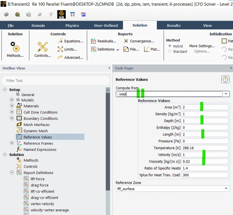
- compute from the inlet of the surface.
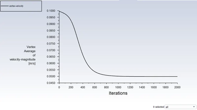
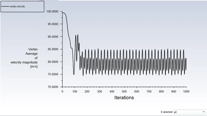
- Vertex velocity plot:
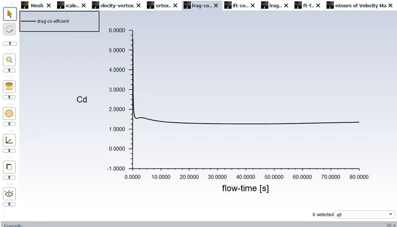
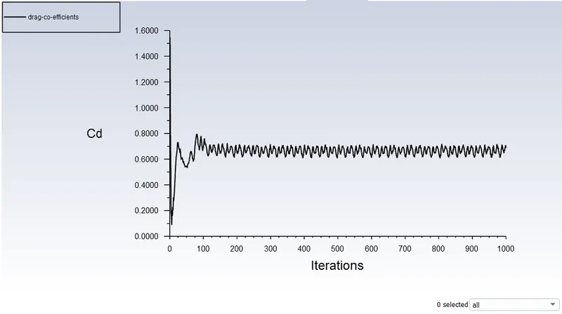
- Co-efficient of drag:
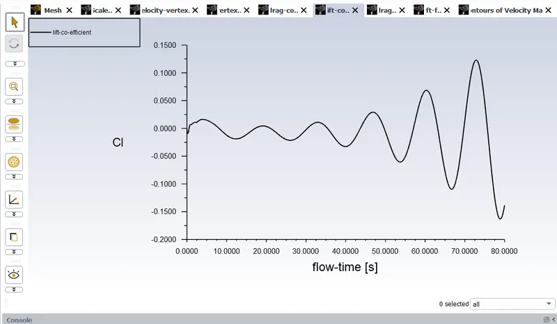
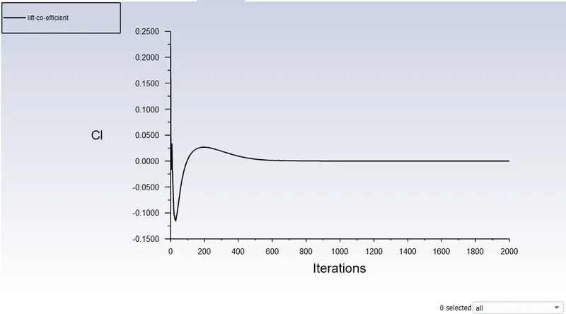
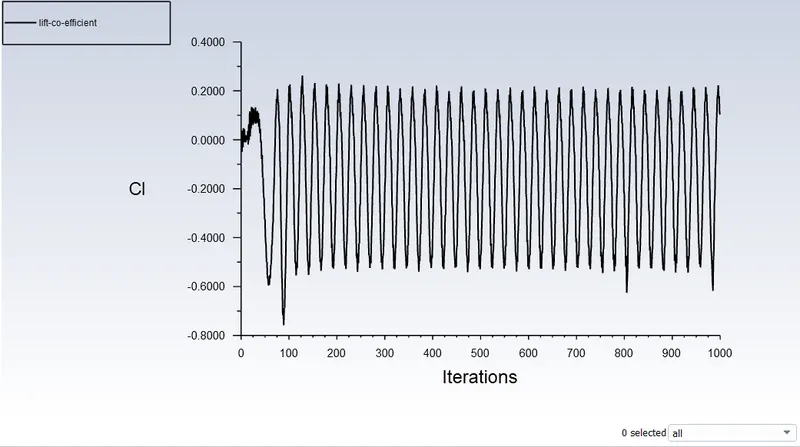
- Co-efficient of lift:
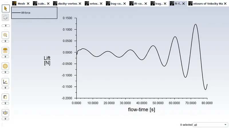
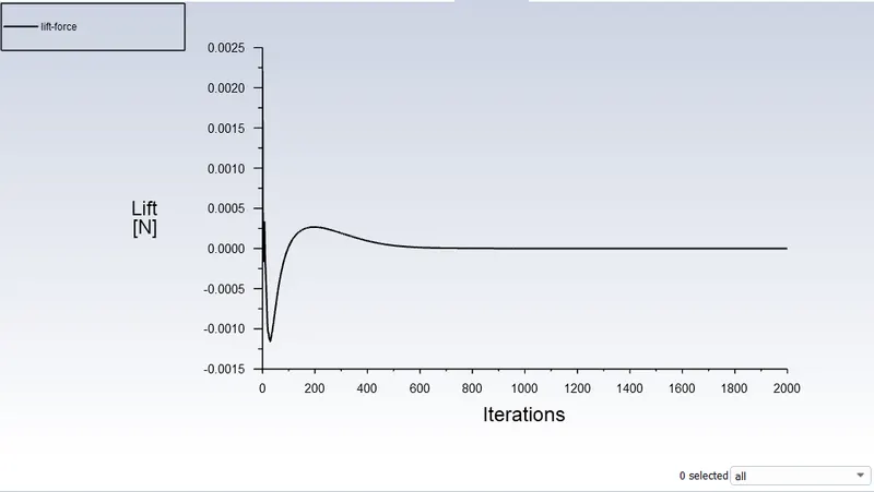
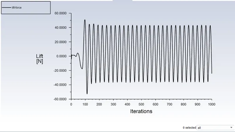
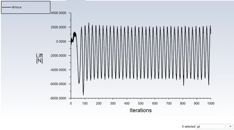
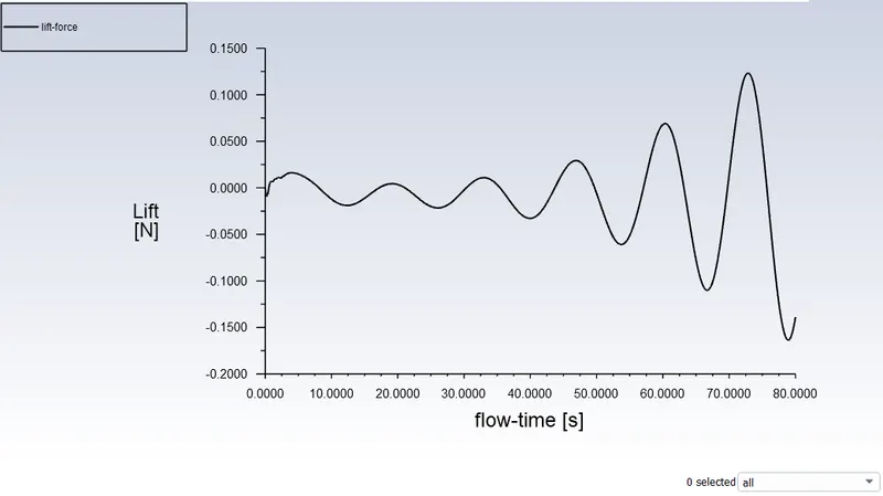
- Lift force:
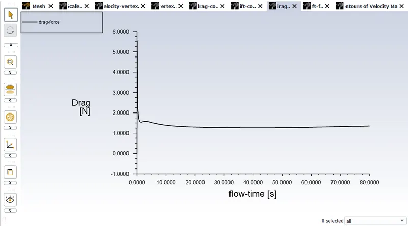
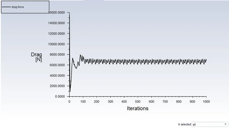
- Drag force:
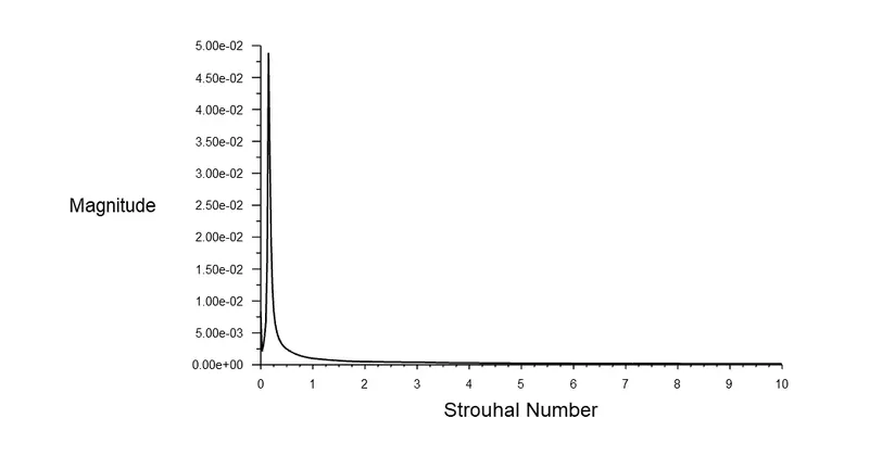
- Strouhal Number:
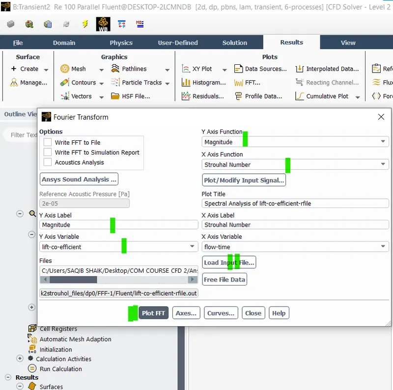
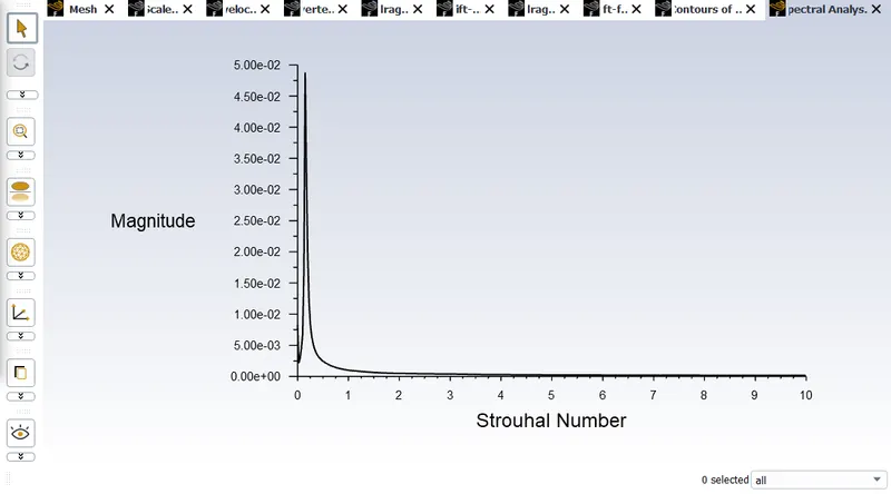
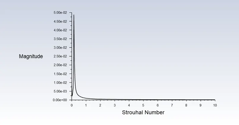
- Strouhal Number at the Reynolds Number 100 is 4.85.
- Steady flow with Re - 10.
- Physical and Boundary conditions:
- Report definitions:
- Drag coefficient and Lift co-efficient:
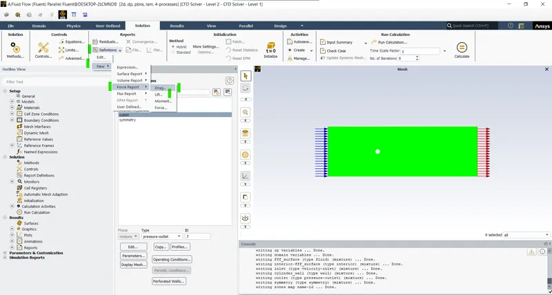
- Creating the moitor point:
- Vetrex average of velocity:
- Reference values:
- Solution methods:
- Contours:
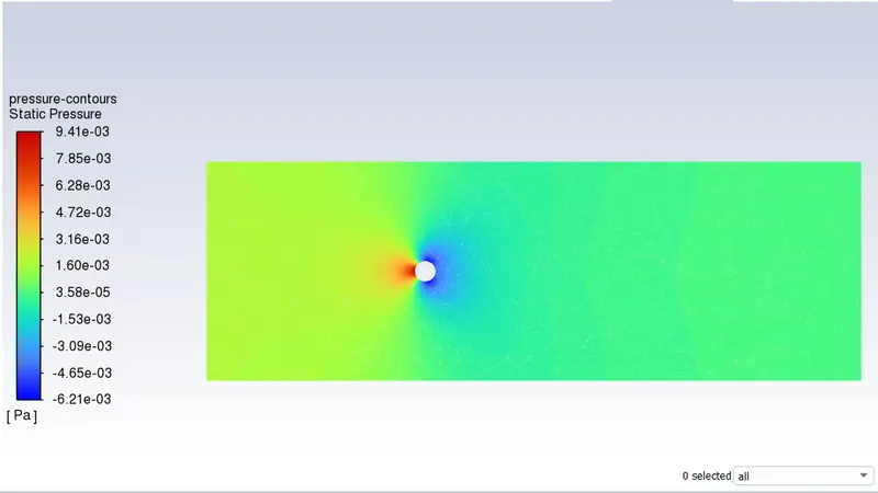
- Pressure contours:
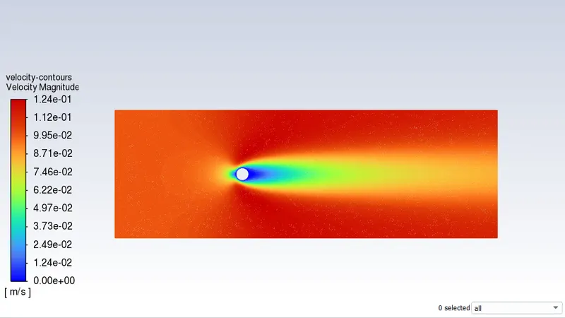
- Velocity contours:
- Animations:
- Velocity contours animation:
- Pressure contours animation:
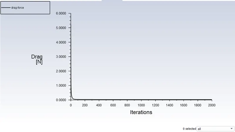
- Drag co-efficient and force:
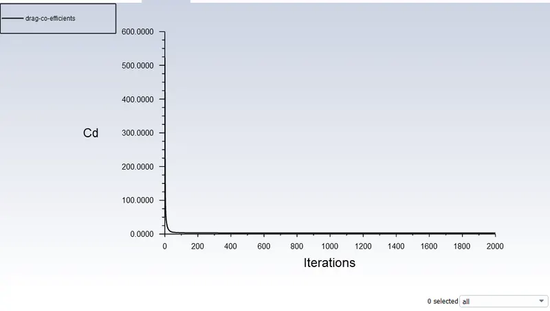
- Drag co-efficient: 3.327
- Lift co-efficient and force:
- Vertex average of velocity:
- Pressure contours:
- Velocity contours:
- Physical and Boundary conditions:
Results:
- Steady state Re:10:
- Residuals:
- Vertex average of velocity:
- Pressure contours:
- Velocity contours:
- Drag co-efficient and force:
- Lift co-efficient and force:
- Residuals:
- Steady state Re:100:
- Residuals:
- Reference values:
- Vertex average of velocity:
- Pressure contours:
- Velocity contours:
- Drag co-efficient and force:
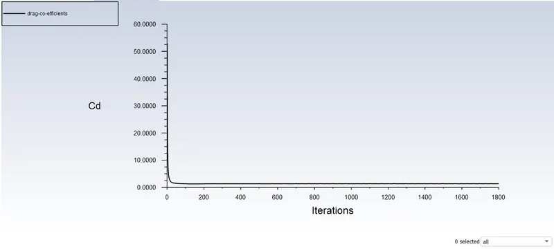
- Drag co-efficient: 1.3592676
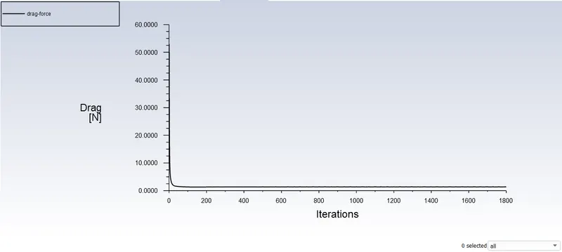
- Lift co-efficient and force:
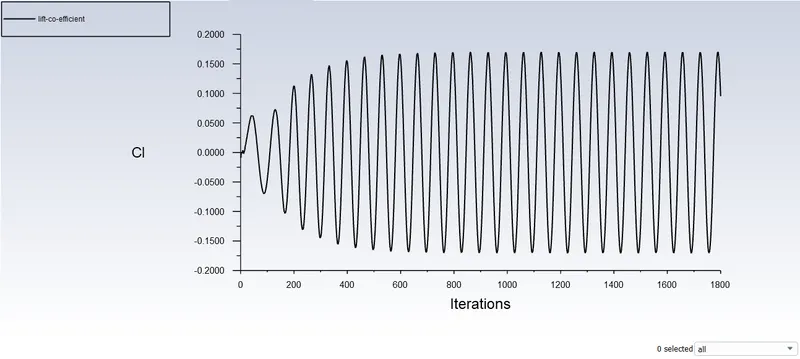
- Lift co-efficient: 0.0951
- Residuals:
- Steady state Re:1000:
- Residuals:
- Reference values:
- Vertex average of velocity:
- Pressure contours:
- Velocity contours:
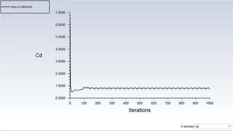
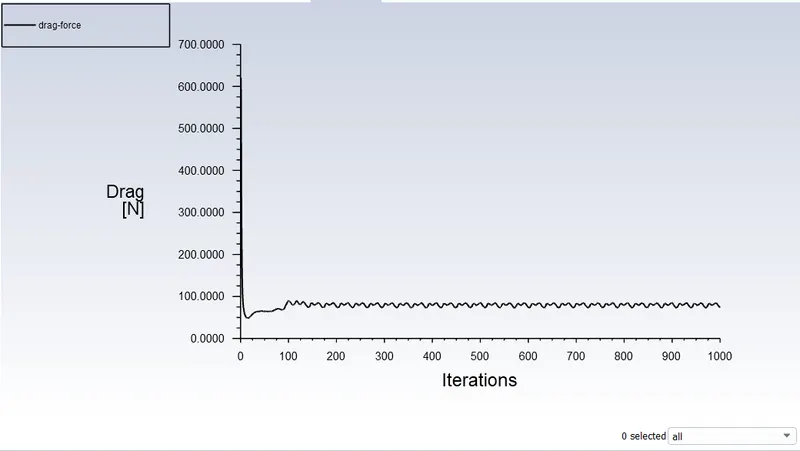
- Drag co-efficient and force:
-
Drag co-efficient: 0.73599219
- Lift co-efficient and force:
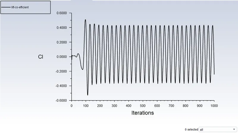
- Lift co-efficient: -0.24391304
- Residuals:
- Steady state Re:10,000:
- Residuals:
- Reference values:
- Vertex average of velocity:
- Pressure contours:
- Velocity contours:
- Drag co-efficient and force:
- Lift co-efficient and force:
- Residuals:
- Steady state Re:1,00,000:
- Residuals:
- Reference values:
- Vertex average of velocity:
- Pressure contours:
- Velocity contours:
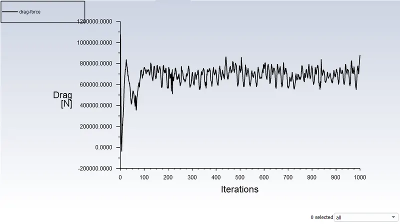
- Drag co-efficient and force:
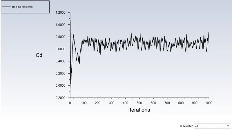
- Drag co-efficient: 0.88
- Lift co-efficient and force:
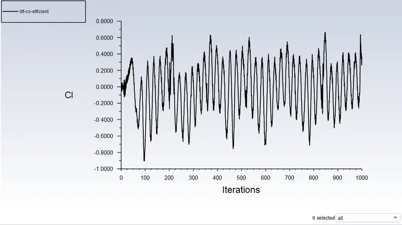
- Lift co-efficient: 0.37
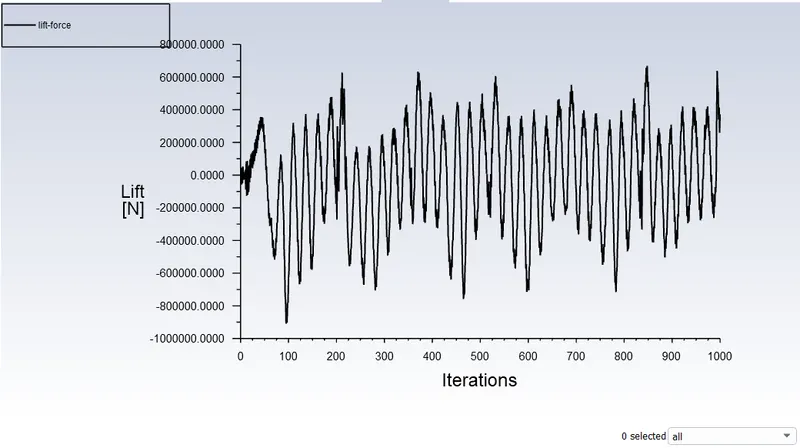
- Residuals:
- Transient state Re - 100(Part-1) Run fo 80sec:
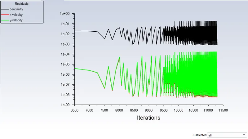
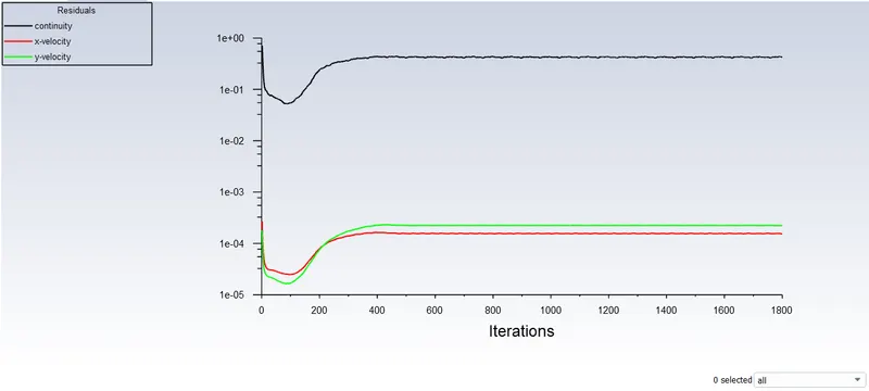
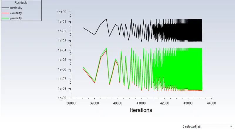
- Residuals:
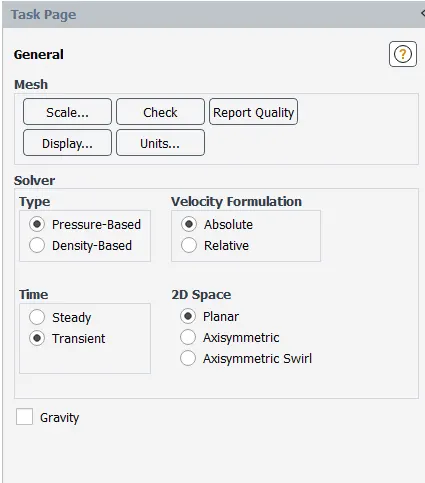
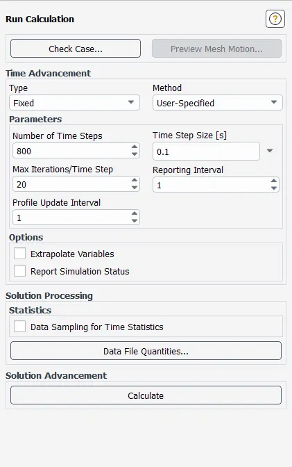
- Run for 800 time step with 0.1 second time step(80 seconds).
- Reference values:
- Vertex average of velocity:
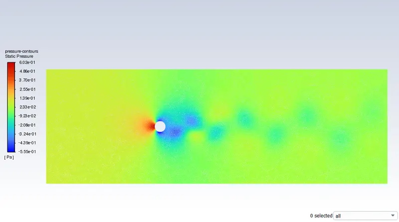
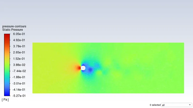
- Pressure contours:
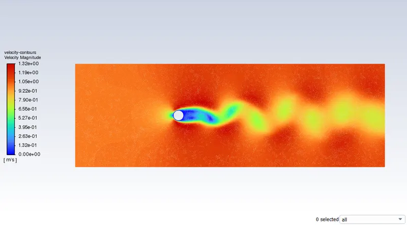
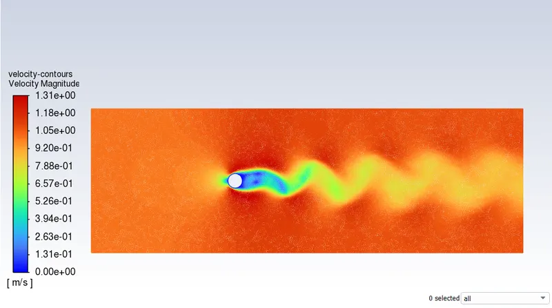
- Velocity contours:
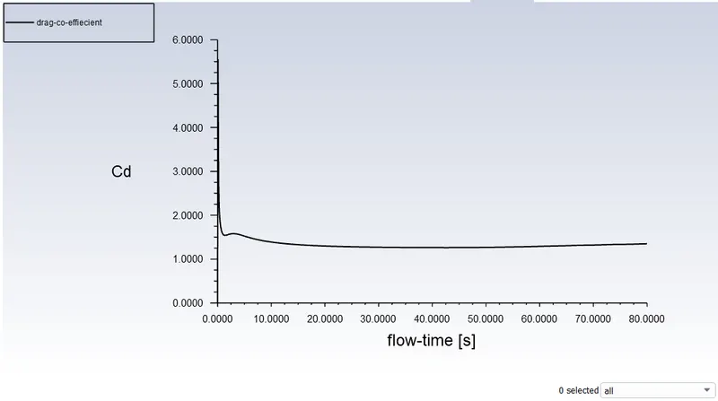
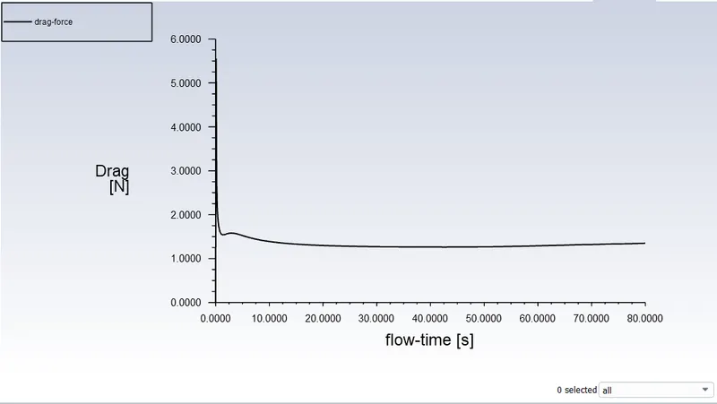
- Drag co-efficient and Drag force:
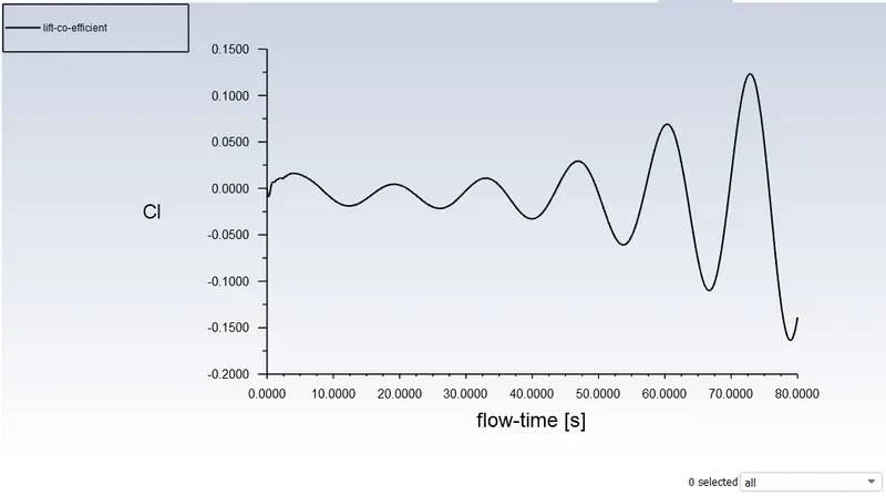
- Lift co-efficient and Lift force:
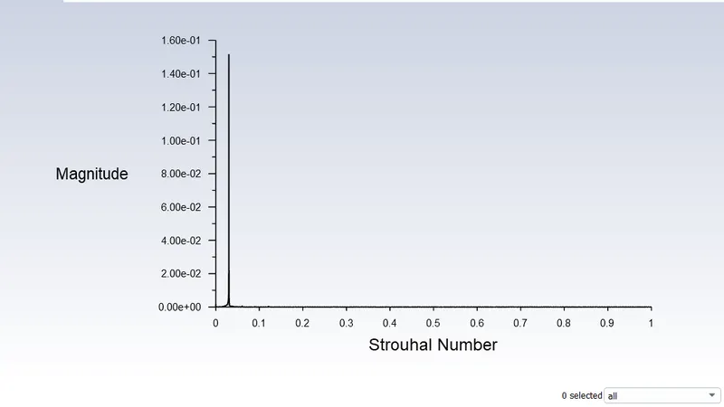
- Strouhal Number:
- Residuals:
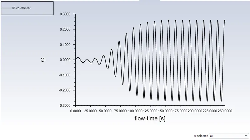
- Transient state Re - 100(Part-1) Run fo 250sec:
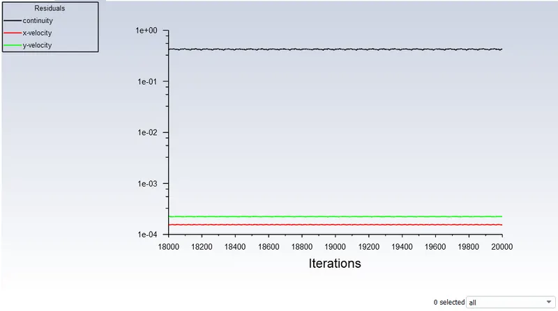
- Residuals:
- Reference values:
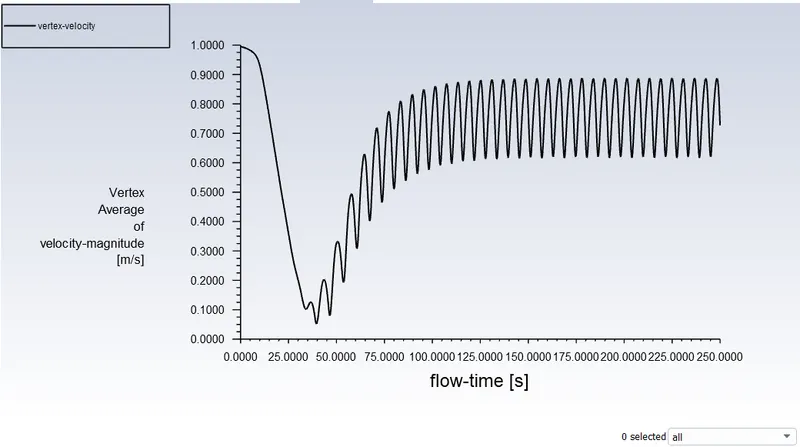
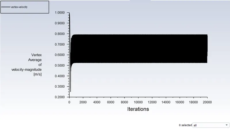
- Vertex velocity:
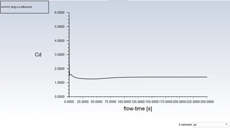
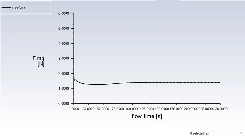
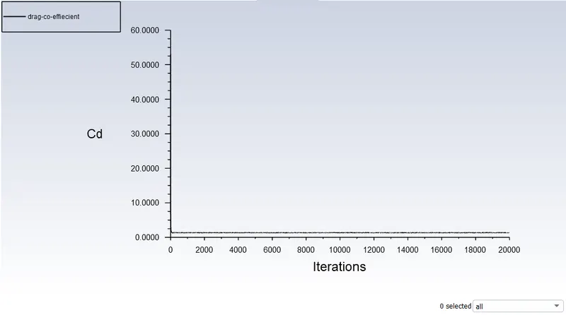
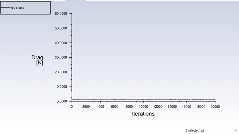
- Drag co-efficient and Drag force:
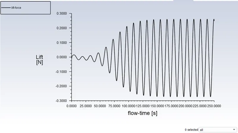
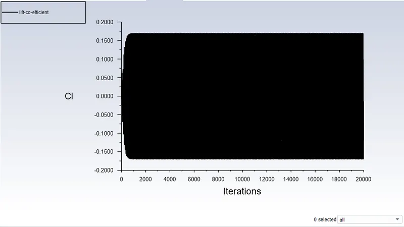
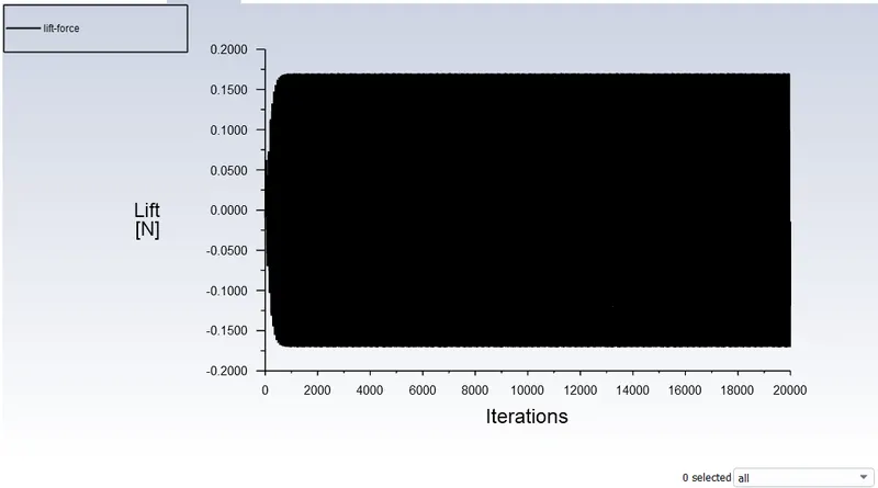
- Lift co-efficient and lift force:
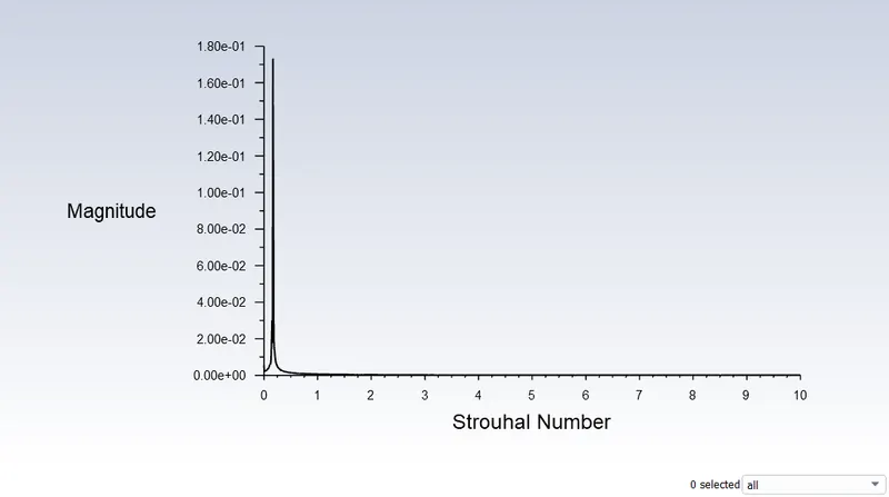
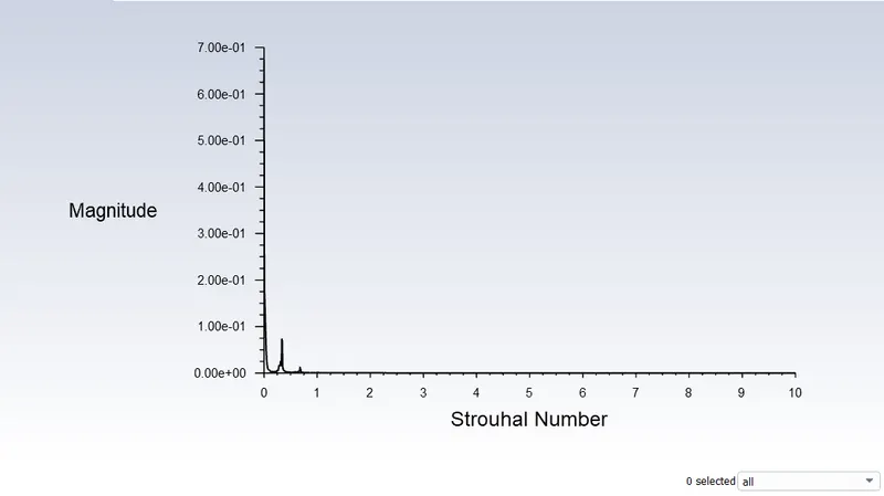
- Strouhaul Number:
- From lift co-efficient:
- From vertex average velocity:
- From lift co-efficient:
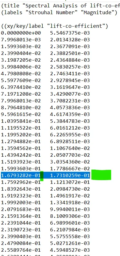
- Here the Strouhaul Number is 0.1679.
- Residuals:
- Steady state Re -100(Part-1):
- Residuals:
- Reference values:
- Vertex average of velocity:
- Drag co-efficint and Drag force:
- Lift co-efficient and Lift force:
- Pressure contours:
- Velocity contours:
- Strouhal Number:
- Residuals:
- Table:
-
Sl.no Flow Reynolds number Velocity (m/s) Drag co-efficient (Cd) Lift co-efficient (CL) 1 Laminar 10 0.1 3.3277026 -3.17E-06 2 100 1 1.3592676 0.095182565 3 1000 10 0.73599219 -0.24391304 4 Turbulent (k-omega SST) 10000 100 0.68670357 0.10279186 5 100000 1000 0.52227227 0.26976789 - Considering the laminar flow:
-
Sl.no Flow Reynolds number Velocity (m/s) Drag co-efficient (Cd) Lift co-efficient (CL) 1 Laminar 10 0.1 3.3277026 -3.17E-06 2 100 1 1.3592676 0.095182565 3 1000 10 0.81571379 0.4243554 4 10000 100 0.65295924 0.10279186 5 100000 1000 0.88037444 0.37250111 - Here as we the flow to be only laminar it shows an anomaly with Re 1,00,000.
- But in several researchs it has shown that for external flow the transition starts at Re1,00,000 and in some it is referred as turbulent so modelling to the conditions we have next the turbulent model.
- Considering the turbulent flow:
-
Sl.no Flow Reynolds number Velocity (m/s) Drag co-efficient (Cd) Lift co-efficient (CL) 1 Laminar 10 0.1 3.3277 -3.2E-06 2 100 1 1.3593 9.5E-02 3 1000 10 0.8157 4.2E-01 4 10000 100 0.6530 1.0E-01 5 Turbulent (k-omega SST) 100000 1000 0.5223 2.7E-01 - Error calculation:
- Taking the Re 1,00,000 for error calculation:
- Therotical value = 0.5
- Numerical value = 0.52
- Error = 4%
- Hence validated.
- For Transient solver(case-1):
-
Sl.no Reynolds number Solver Time step size/No of steps Run Time (sec) Drag coefficient Lift coefficient 1 100 Transient Solver 0.1/2500 25 1.4038588 0.24782287 2 100 Steady state 20000 iter 1.359 0.08 - Here for Reynolds Number 1,00,000 we need to run the simulation with turbulent model (k-omega SST) as the transition begins in this range from laminar to turbulent.
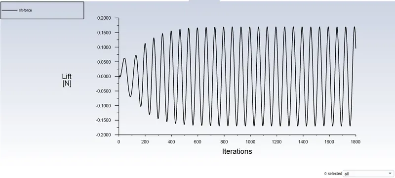
- As the vortices are formed the lift and drag force and co-effcient vary when the flow seperation takes place it creates regions of low and high pressure which cause repeating variations in the lift and drag, some of the values are listed below.
-
Reynolds number Lift Force variation Lift co-efficient varition 10 Stable Stable 100 -0.174 to 0.174 -0.174 to 0.174 1000 -38 to 43 -0.38 to 0.43 10000 -5300 to 2100 -0.51 to 0.2 100000 -7,00,000 to 7,00,000 -0.7 to 0.7
-
- Graph (Reynoldds Number vs Drag co-efficients):
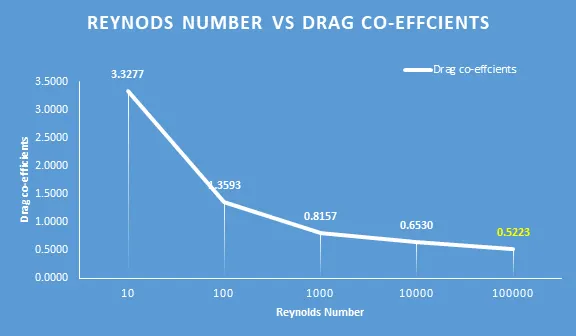
- It can be clearly observed from the graph that as the Reymolds number increases drag co-efficient decreases.
- Video-animation links:
-
Sl.no. Case Iteration Solver Type Reynolds Number Links 1 1 0.1sec/2500 times Transient 100 Re 100 Transient 2 2000 Steady 100 Re 100 Steady 3 2 2000 Steady 10 Re 10 4 2000 Steady 100 Re 100 5 2000 Steady 1000 Re 1000 2000 Steady 10000 Re 10 000 2000 Steady 100000 Re 1 00 000
-
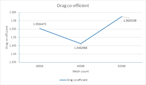
- Grid Independency study was done and the erorr with consigative values is 1.4%, so we can proceed:
Conclusions:
- The simulations are successfully conducted and the results obtained are inaccordance with the research work.
- The procedure and the comparision done are explained in detail.
- As the Reynolds number increases the drag co-efficient decreses.
- The Strouhal Number for the Reynolds number 100 is 0.1679 with magnitiude of 0.173
- The challenge/project results are throughly backed by the Literature survey (both experimental and Numerical) only after complete and detailed study and investigation of the researched materials, these are provided below in reference section.
- For the convergence criteria the drag co-efficients along with residuals are inspected (Stable or repeating pattern fully developed).
References:
- David E. Alexander,
Chapter 3 - Fluid Biomechanics,
Editor(s): David E. Alexander,
Nature's Machines,
Academic Press,
2017,
Pages 51-97,
ISBN 9780128044049,
https://doi.org/10.1016/B978-0-12-804404-9.00003-7
(https://www.sciencedirect.com/science/article/pii/B9780128044049000037) - Shubham Jain,Nekkanti Sitaram,and Sriram Krishnaswamy.Effect of Reynolds Number on Aerodynamics of Airfoil with Gurney Flap,https://doi.org/10.1155/2015/628632
- Kartik Chandra Bhagat, Subrato Kumar Soren, Sunil Kumar Chaudhary,EXPERIMENTAL AND NUMERICAL ANALYSIS OF DIFFERENT AERODYNAMIC PROPERTIES OF CIRCULAR CYLINDER,https://www.irjet.net/archives/V3/i9/IRJET-V3I9203.pdf
- James Venning, Thomas McQueen, David Lo Jacono, David Burton, Mark Thompson, John Sheridan,
Aspect ratio and the dynamic wake of the Ahmed body,
Experimental Thermal and Fluid Science,
Volume 130,
2022,
110457,
ISSN 0894-1777,
https://doi.org/10.1016/j.expthermflusci.2021.110457. - L. Skrbek, W.F. Vinen,
Chapter 4 - The Use of Vibrating Structures in the Study of Quantum Turbulence,
Editor(s): M. Tsubota, W.P. Halperin,
Progress in Low Temperature Physics,
Elsevier,
Volume 16,
2009,
Pages 195-246,
ISSN 0079-6417,
ISBN 9780080548104,
https://doi.org/10.1016/S0079-6417(08)00004-8. - Aziz, Elsayed & Esche, Sven & Chassapis, C.. (2008). Online Wind Tunnel Laboratory. 10.18260/1-2--3402.
- Mallick, Monalisa. (2016). VARIATION OF DRAG COEFFICIENT ON ROUGH CYCLINDRICAL BODIES. 10.13140/RG.2.1.3202.3926.