Week 3 - External flow simulation over an Ahmed body.
External flow simulation over an Ahmed body
Aim: - To perform external flow simulation on Ahmed Body using ANSYS Fluent.
Introduction
Ahmed body: -
Ahmed body is a model which has an aerodynamic shape similar to a real automobile. Ahmed body is used for the validation of vehicle aerodynamic simulation. Based on experimental data of various parameters like lift coefficient, drag coefficient, pressure and velocity distribution over the surface of the body and in the wake region, etc. Ahmed body helps in developing and redesigning the prototype model of a real vehicle.
Ahmed body was created by S.R. Ahmed and published about it in his research paper “Some Salient Feature of the Time-Averaged Ground Vehicle Wake” in the year 1984. Since then, it is used as a benchmark for validation tools for aerodynamic simulation of automobiles. With the increase in computing power, the development process of automobiles is mostly about optimization digitally. It helps in decreasing development time and cost. Also, optimization of an automobile leads to manufacturing efficient automobiles with minimum fuel consumption, less emission, and better driving stability. Experimental data obtained from an experiment on the actual Ahmed body is used as a reference to validate the simulation.
Problem Definition:-
In this project. We will perform a CFD analysis of Ahmed body using ANSYS Workbench.
The geometry is designed using ANSYS Space Claim, the mesh will be generated using ANSYS Meshing and the problem is solved using ANSYS Fluent.
Our goal in this project is to compute the drag coefficient and to compare it with experimental data. Along with that, we will obtain the velocity and pressure contour to observe the fluid in the wake region and at the point of separation.
Procedure
Workbench Project
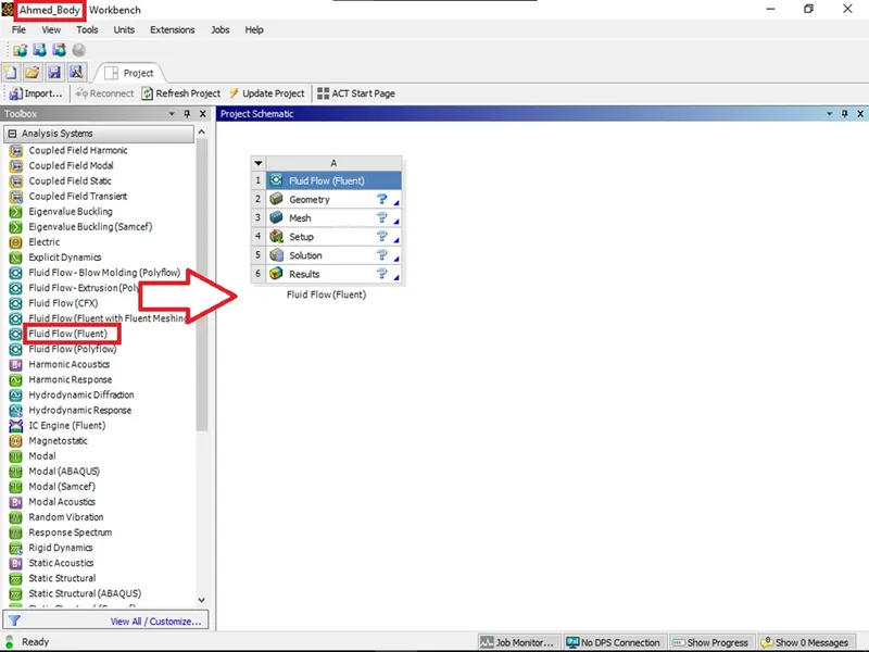
Start ANSYS Workbench and drag and drop Fluid Fluent into the main window and save it as Ahmed_Body.
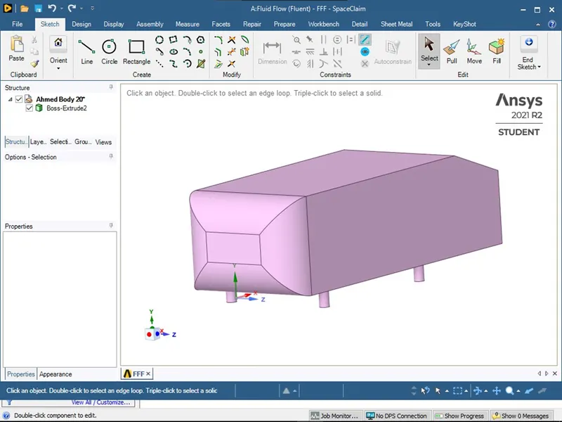
The geometry of Ahmed Body with Space Claim
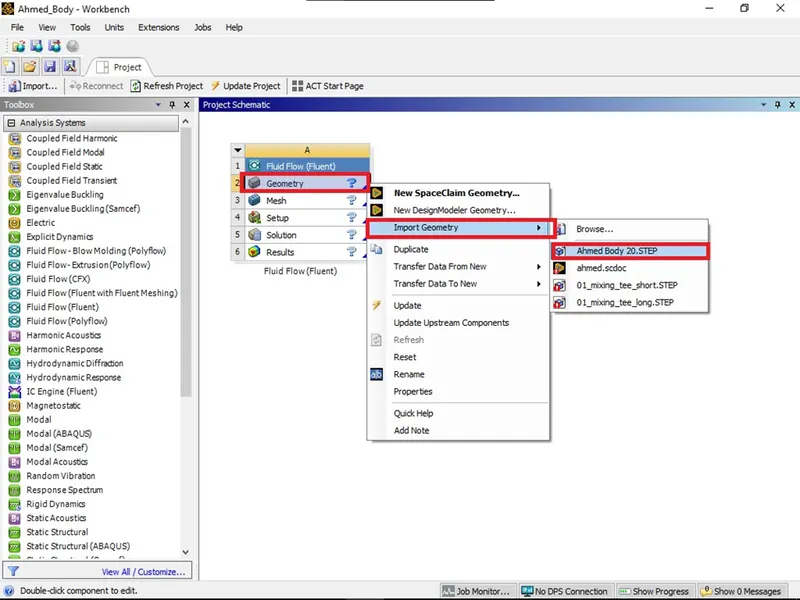
-Right-click on Geometry and click on Import Geometry and select the file of Ahmed body that is already downloaded.
-Double click on Geometry. Space Claim will open with Ahmed body loaded in it.
- Since Ahmed body is perfectly symmetrical, we can simulate the half body. To split the Ahmed body, Click on the Design tab and click on the Plane icon. Select the Coordinate axis to produce the Coordinate Plane.
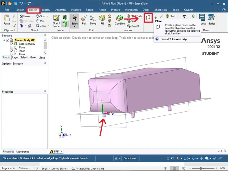
-On the Structure tab, uncheck the planes to hide the planes.
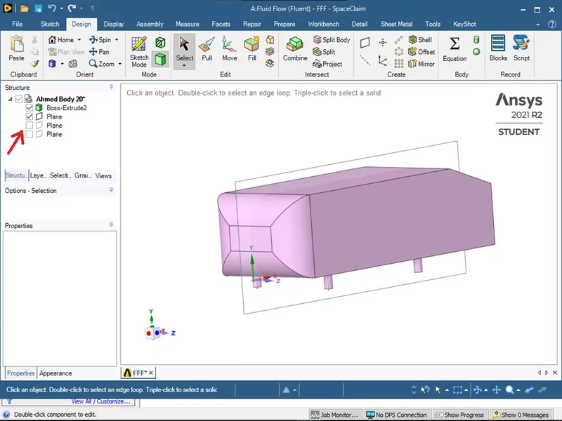
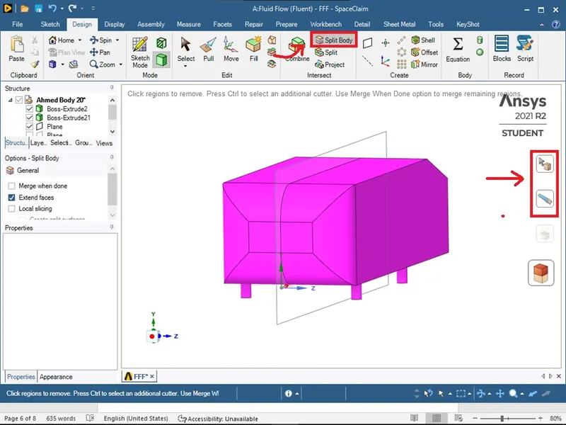
-Click on the Design tab and click on the Split Body icon. Select the target body as Ahmed Body and Select Plane to cut the Ahmed body. Two bodies are created – Boss-Extrude2 and Boss-Extrude21.
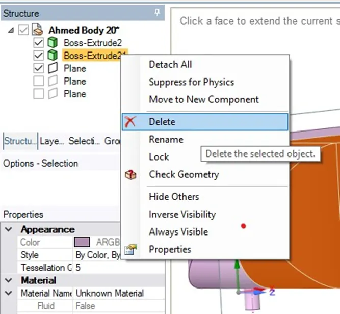
-Delete the Second Half of the Body. On the Structure tab, Right-click on Boss-Extrude21 and click on delete
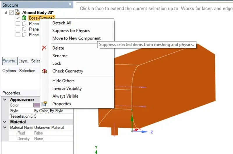
-Suppress for Physics of remaining Half of the Body. Right-click on Boss-Extrude2 and click on Suppress for Physics.
-We have Prepared the Geometry of the Ahmed Body. Now we have to create an external enclosure to simulate external aerodynamics around the body. This enclosure starts with 2m before the body and extends 5m behind the body.
-Click on the Prepare tab and click on the Enclosure icon. Untick on Symmetric dimension.
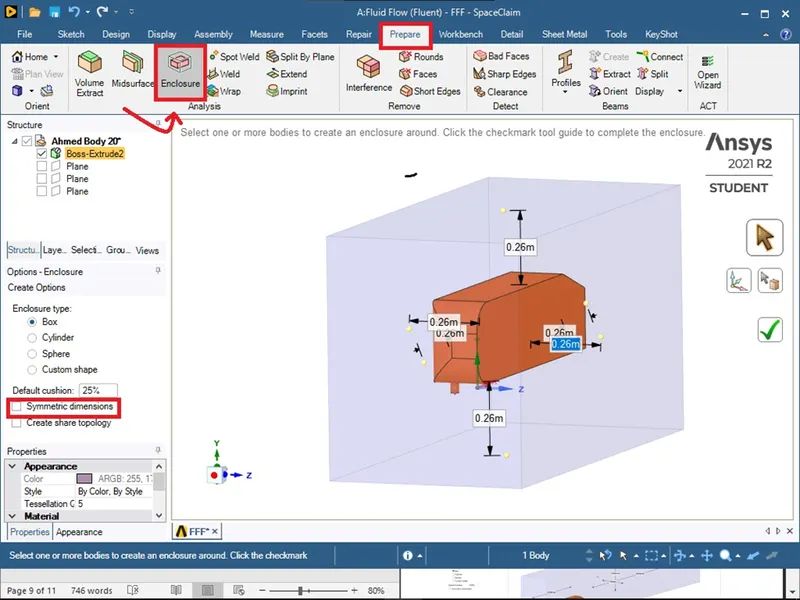
-Enter the dimensional details of the enclosure as shown in the below figure
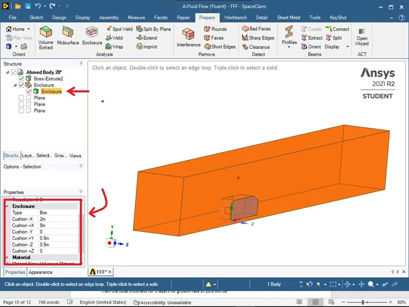
But to produce refined mesh close to Ahmed body, we need to create another enclosure which starts 0.4m before Ahmed body and 1m behind the body. Dimensional detail of Enclosure2 in the below figure.
-Repeat the previous step with new dimensional values
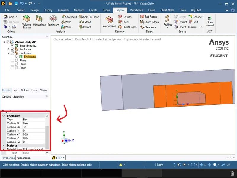
- After creating an enclosure within the enclosure, we can observe the overlapping of the two-enclosure box.
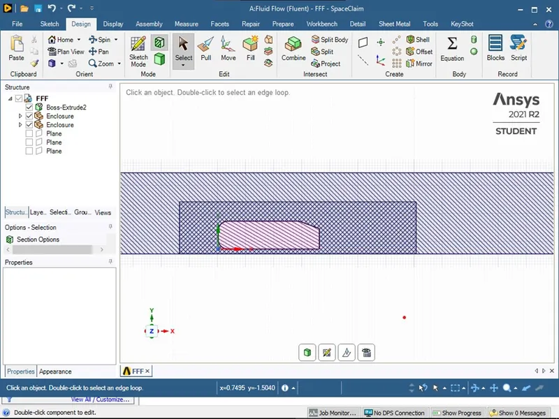
-To eliminate this overlapping. Click on Prepare tab and click on the Inference icon. It will automatically detect the overlapping bodies and subtracts the interference volume from the larger enclosure
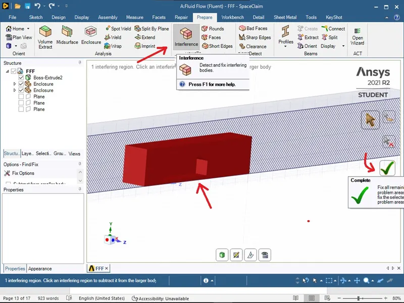
-. Click on the Right icon to complete the process. We can see no overlap in between.
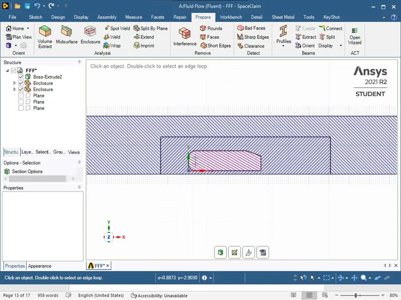
-Click on File and click on Save Project and Close the Space Claim.
Next, we start meshing using ANSYS Meshing.
Meshing with ANSYS Meshing
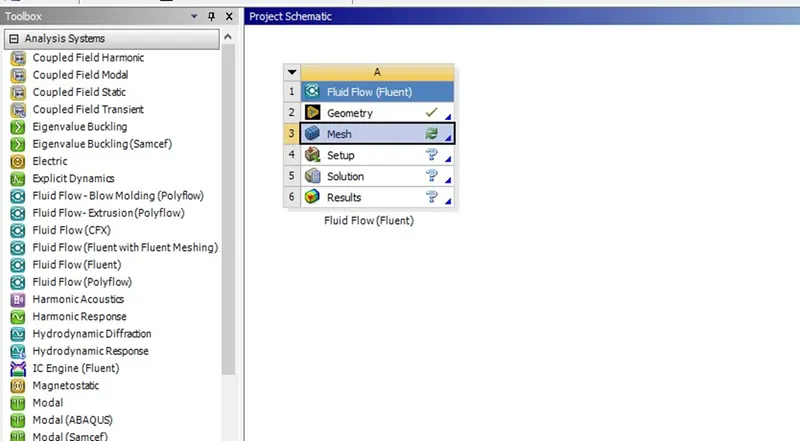
In the Workbench, double click on Mesh to open ANSYS Meshing.
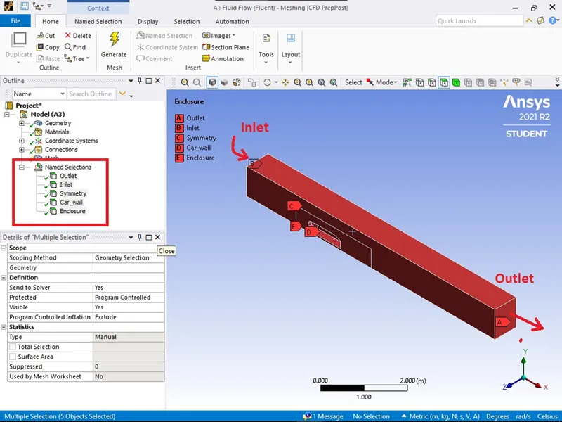
-Assign Name to the faces in the Model. Select the face by clicking on the face and then press “N” on the keyboard, a dialog box of Selection Name opens. Type the name of the selected face. Repeat the same step for all the faces in the model.
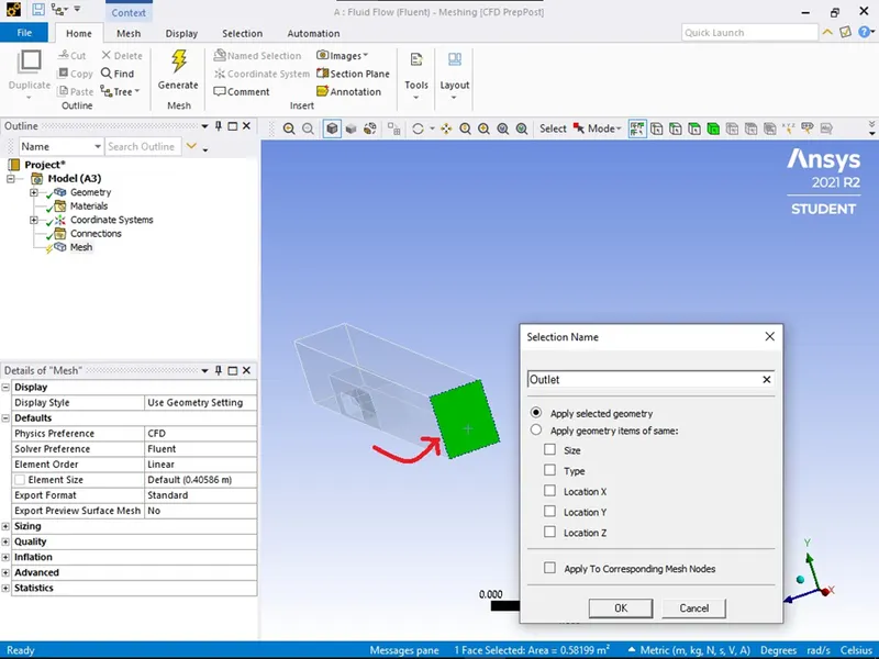
For the selection of multiple faces press and hold the control key and click on faces to be selected. For the surface of Ahmed Body, click on Select Mode-->Box Select, to select all its patches.
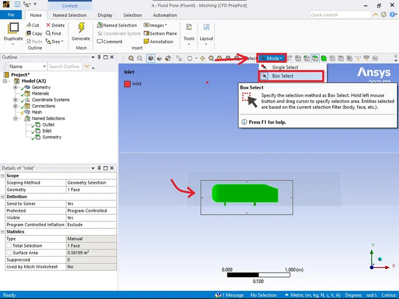
-To hide faces, select the face and press F8. To unhide it press Shift+F8.
Make sure that all the faces are named. Check it under the Outline tab à Project àModel àNamed Selection.
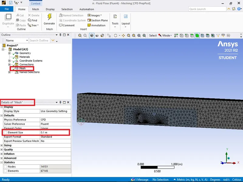
-Under the Outline tab --> Project à Model --> Mesh, in the Details of Mesh specify the Element Size (100mm).
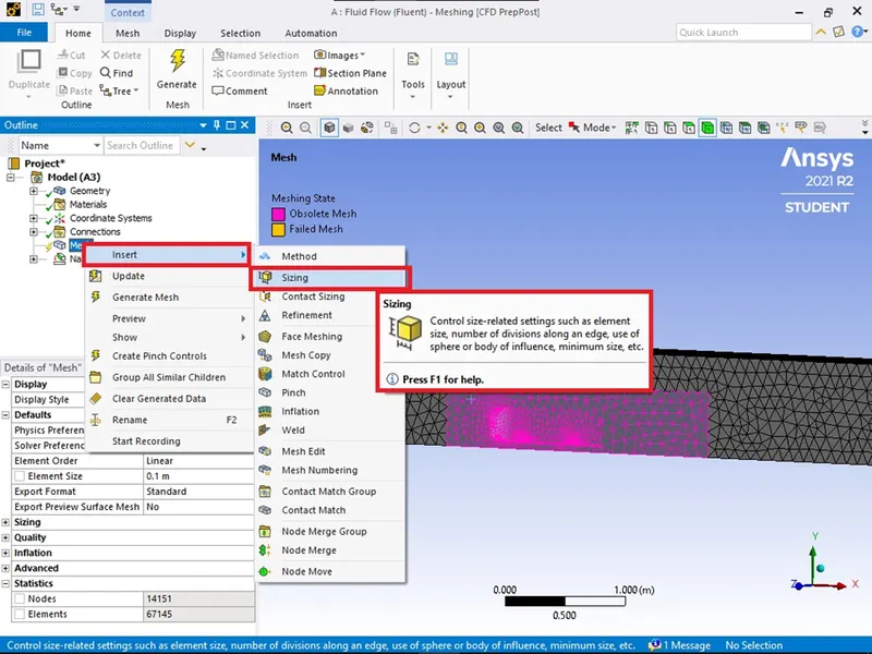
- Under the Outline tab à Project à Model à Mesh, Right-click on Mesh and Click on Insert à Sizing.
-In the Detail of “Sizing”-Sizing à Geometry. Select the inner enclosure body and click on Apply in the Geomety tab. For Type select Element Size and specify the Element Size (50mm).
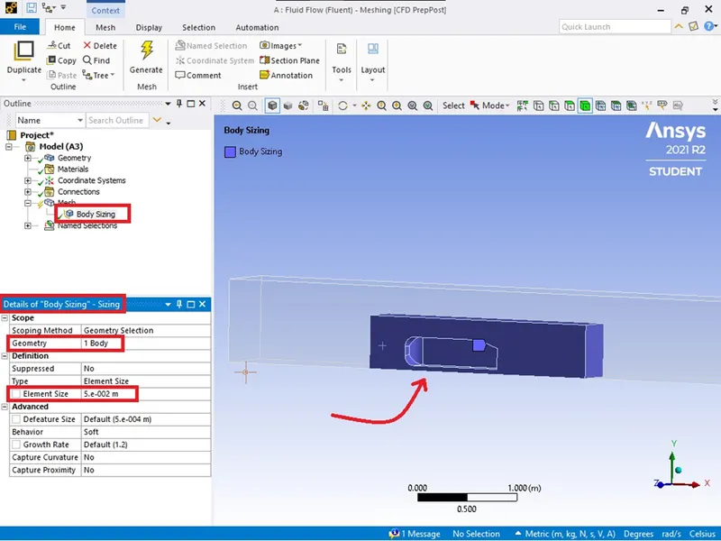
- Calculation of First Layer Thickness for Inflation Layer
Since the flow is turbulent, using y+ we will calculate the first cell height
Input: Y+ = 30
Free Stream Velocity = 25 m/s
Dynamic Viscosity = 1.7894e-05 kg/m-s (Air)
Density = 1.225 kg/m3 (Air)
Calculation In Jupyter Notebook
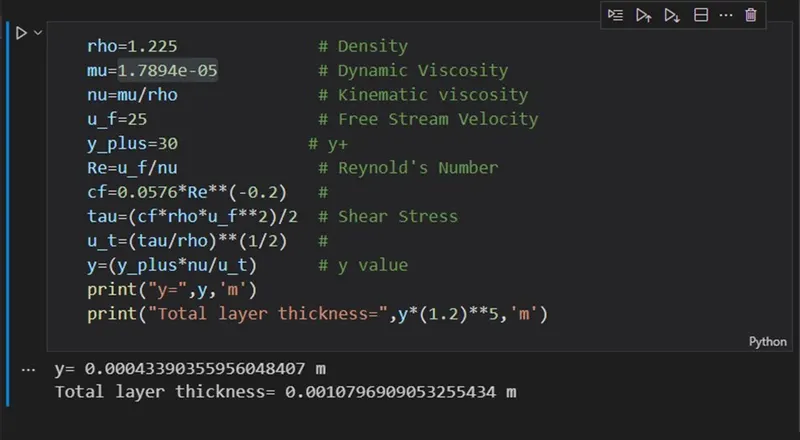
Then the total thickness for 5 layers for growth rate of 20% will be
Total Thickness = (4.339e-04) *(1.2) ^ (5-1) =0.107mm
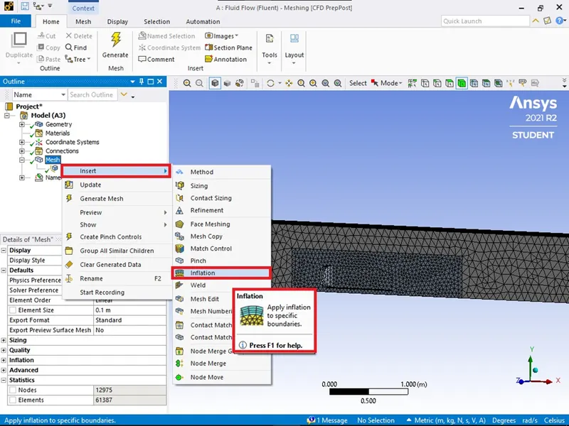
- We need to add an inflation layer near the Car_Wall surface. Under the Outline tab à Project à Model à Mesh, Right-click on Mesh and click on Insert à Inflation.
- In the Details of “Inflation” à Geometry tab, select the inner enclosure. In the Boundary Scoping Method tab select Named Selection. In the Boundary tab select Car_Wall as the boundary for the inflation layer.
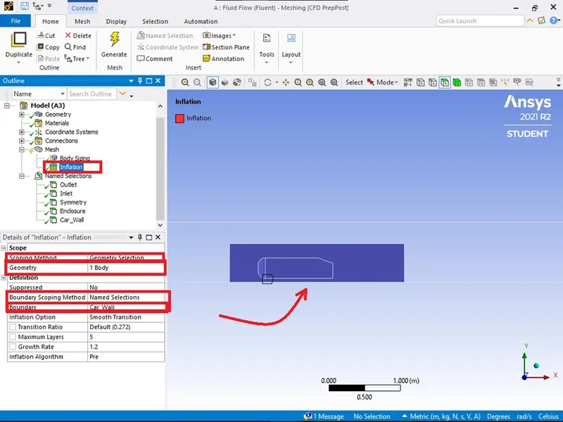
- In the Detail of “Inflation”- Inflation, Inflation Option tab à Total Thickness. Specify No. of Layers as 5, Growth Rate as 1.2, and Maximum thickness as 1.07e-03 m.
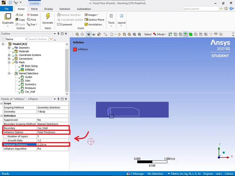
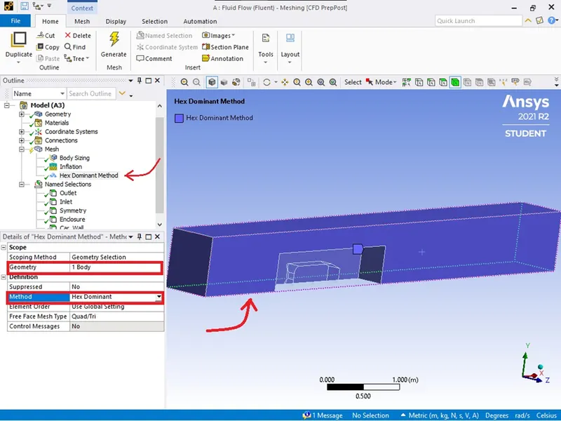
- Similarly Under the Outline tab à Project à Model à Mesh, Right-click on Mesh and click on Insert à Method.-In the Details of “Method” à Scoping Method tab, select the outer enclosure body and click on the application. For Method select Hex Dominant
-To generate mesh, click on Generate icon.
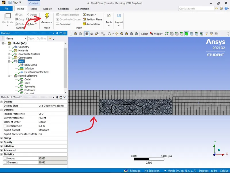
The meshing is completed. Click on File à Save Project to save the mesh in Workbench and close the ANSYS Meshing.
-in Workbench right-click on Mesh à Update to update the mesh in the Workbench.
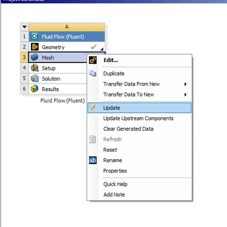
Setup of Problem in ANSYS Fluent
-In Workbench, double click on Setup to launch ANSYS Fluent.
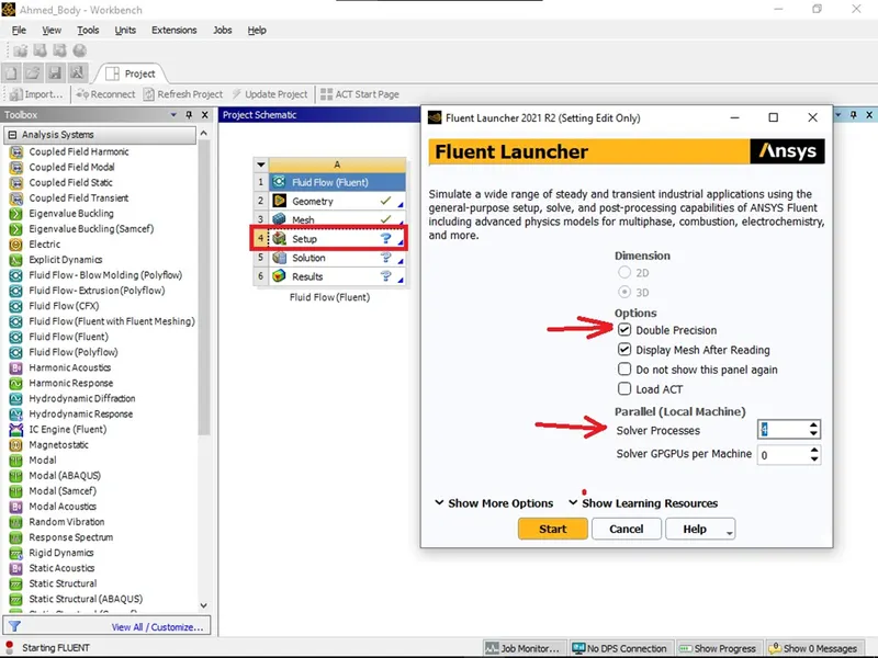
-In the Fluent Launcher Window, check the Double Precision and Solver Process to 4.
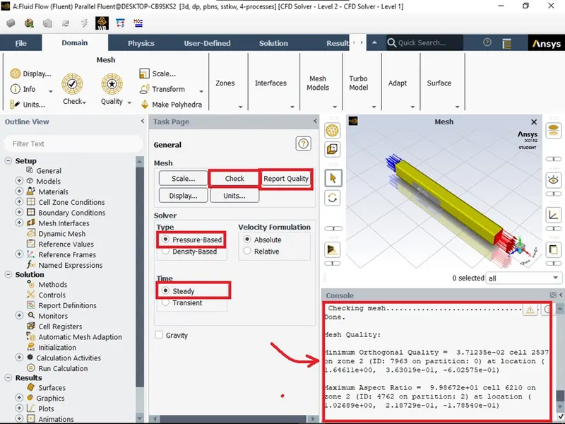
-Under the General tab, Check and Report Quality to check the mesh quality and marked the setting in the below figure.
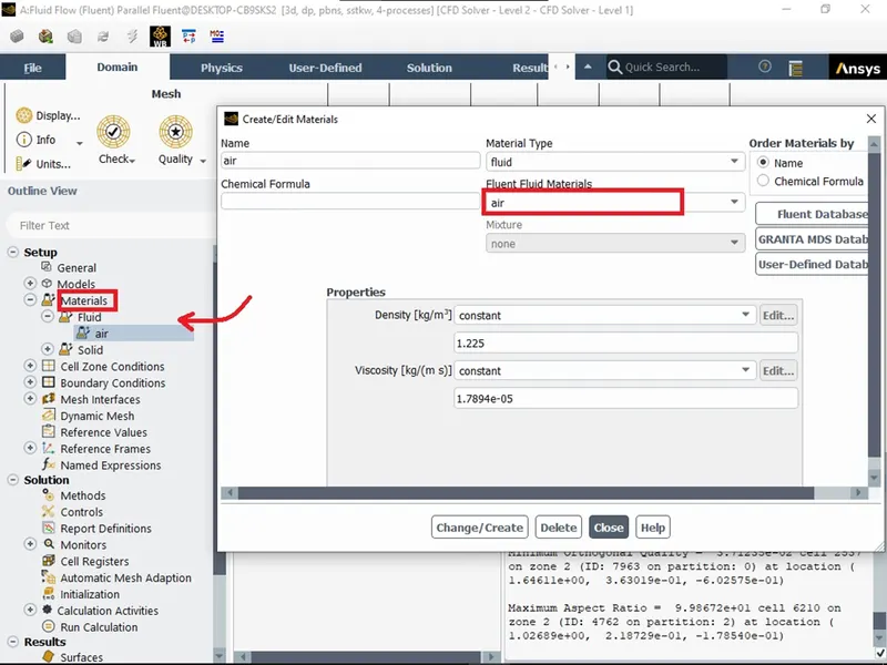
-Under the Setup à Model, double click on Viscous to specify the k-omega(2-equation) model with SST. Under Setupà Material à Fluidà air, specify material as air and check the density and viscosity of the material. Click on Change/Create and close the Create/Edit Material window.
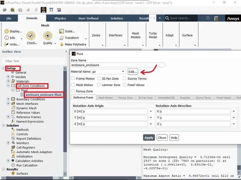
-Setupà Cell Zone Condition à Fluid, double click on enclosure_enclosure to check that enclosure is filled with air.
-Setup à Boundary Condition à Inlet, double click on inlet (velocity) specify the velocity of magnitude as 25 m/s.
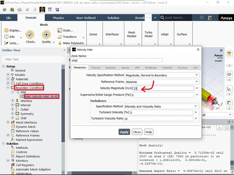
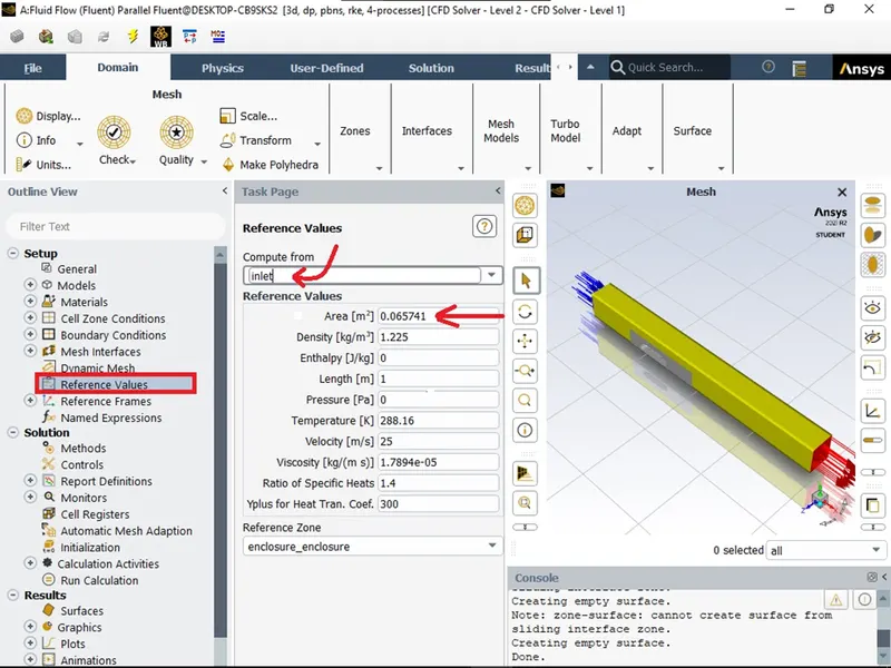
-Under the Setup tab, double click on Reference Value and specify inlet under Compute from and 0.065741 m^2 as Area.
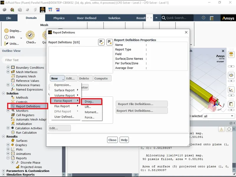
-Under Solution à Report Definitions à New à Force Report à Drag to create a drag report.
-Under Drag Report Definition specify the file name as ‘drag coefficient’, Report Output Type as drag coefficient, and Zones as Car_Wall. Click on ok and close the window.
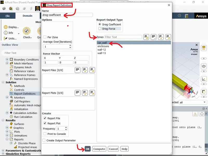
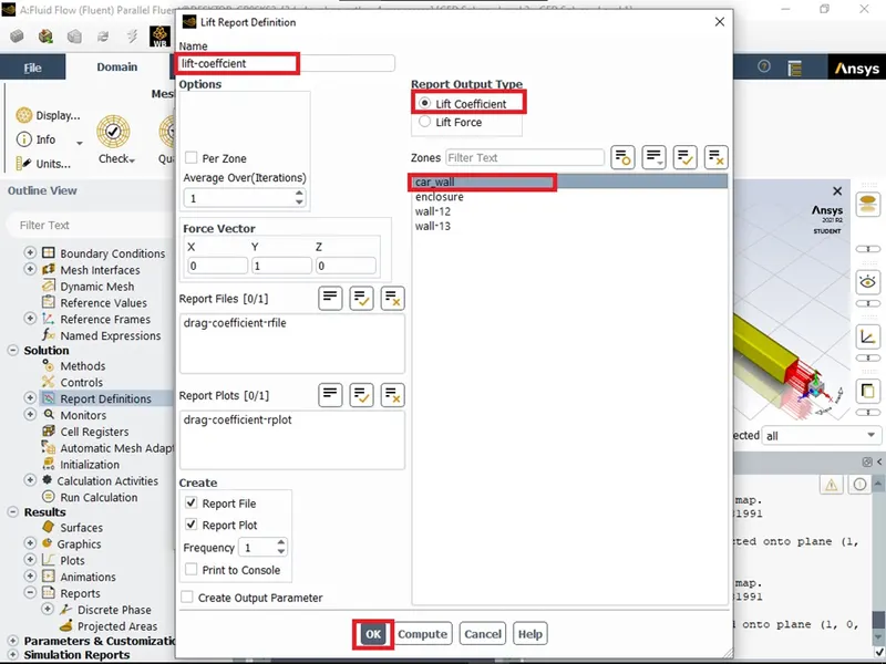
-Repeat the previous process to create a Lift Report Definition.
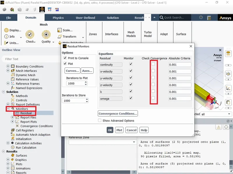
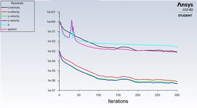
-Under Solution àMonitor, double click on Residual and uncheck the Check Convergence condition as we will specify the fixed number of iterations.
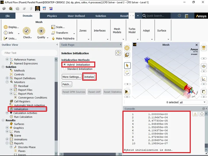
-Under Solution, double click on Initialization select Hybrid Initialization and click on Initialise.
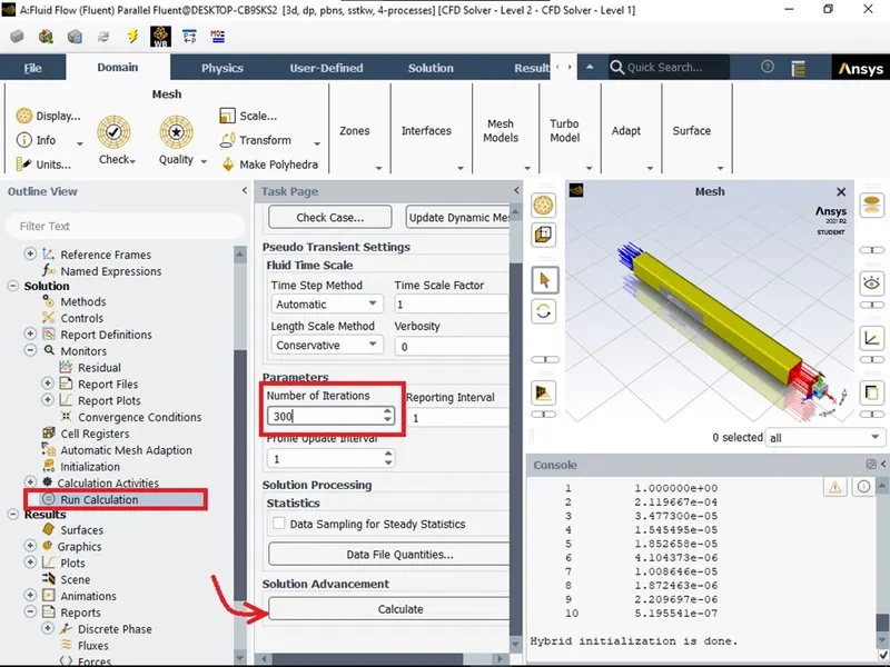
-Under the Solution tab, double click on Run calculation, specify the number of iterations as 300 and click on Calculate to run the calculation.
Results/Outcome
-Residual plot after 300 iteration
-Drag Coefficient plot after 300 iterations.
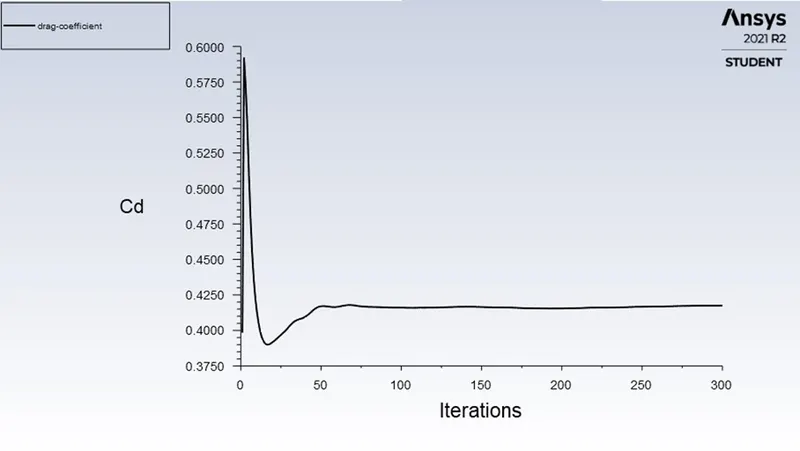
The average drag coefficient of Ahmed Body for the above simulation is 0.417. The results obtained are inaccurate as the grid size is coarse. We need to perform the same simulation for finer grids
In Grid Independence Test, we will run the same simulation with different element size
|
Grid size |
No. of Elements |
No. of Nodes |
Drag Coefficient |
Lift Coefficient |
|
|
Case 1 |
Outer Enclosure: 100mm Inner Enclosure: 50mm |
39798 |
14061 |
0.41749219 |
0.24247851 |
|
Case 2 |
Outer Enclosure: 80mm Inner Enclosure: 30mm |
163275 |
43401 |
0.3747042 |
0.31214487 |
|
Case 3 |
Outer Enclosure: 50mm Inner Enclosure: 20mm |
511463 |
133144 |
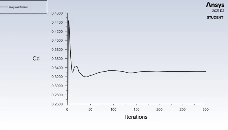
0.33226446 |
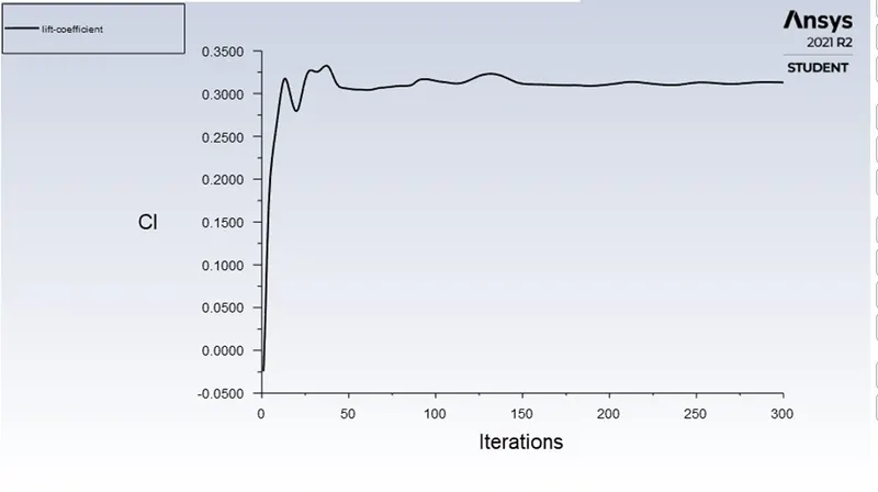
0.3007722 |
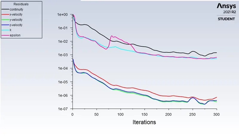
Plots For Case 3 (Fine Grid Size)
Residual Plot
Drag Coefficient Plot
Lift Coefficient Plot
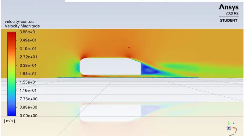
Velocity Contour
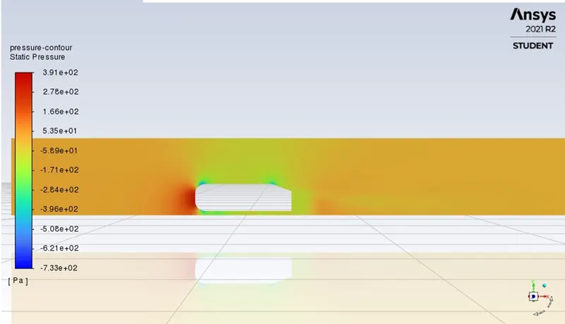
Pressure Contour
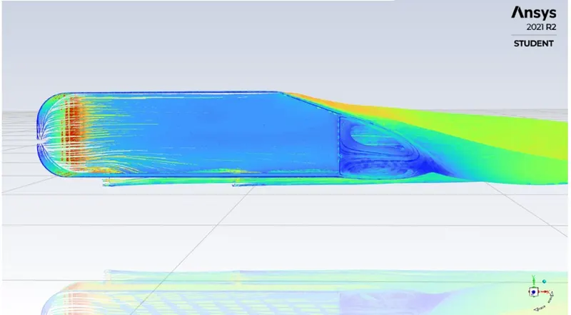
Streamline Plot
Conclusion
We observed negative pressure in the wake region. It is because of the formation recirculation zone in the wake region. Fluid in the rear side of the Ahmed body possesses turbulent kinetic energy that causes force acting on the Ahmed Body. This force leads to negative pressure on Ahmed Body. This negative pressure sucks up the surrounding fluid causes an increase in the drag.
Apart from the wake region, we can observe a small recirculation zone at the curve of the front side and the slant edge on the rear side. This is because of the point of separation. When the fluid detached from the surface of the body, there causes a sudden drop in velocity near that region leads to turbulence and the formation of a recirculation region.