Week 10 - Simulating Combustion of Natural Gas.
Simulation of Combustion of Natural Gas
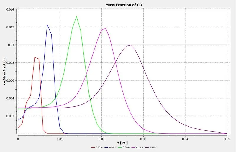
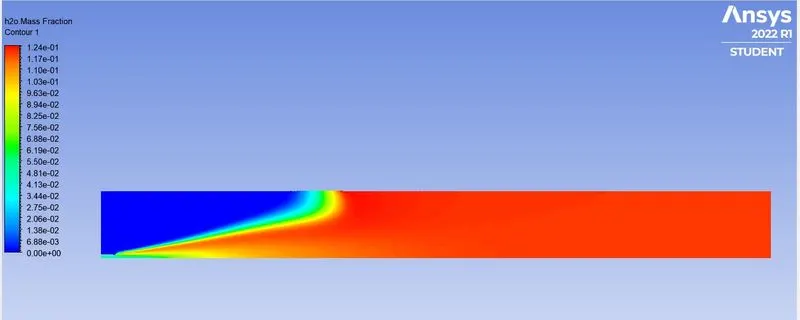
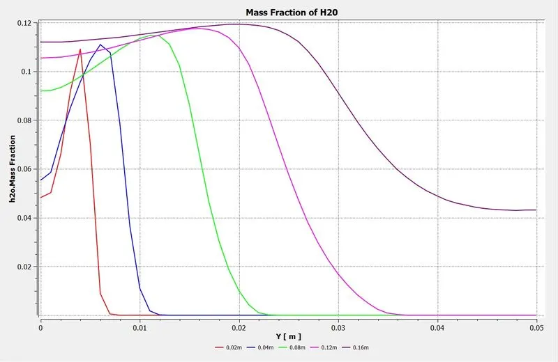
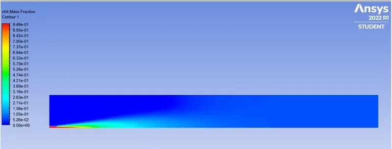
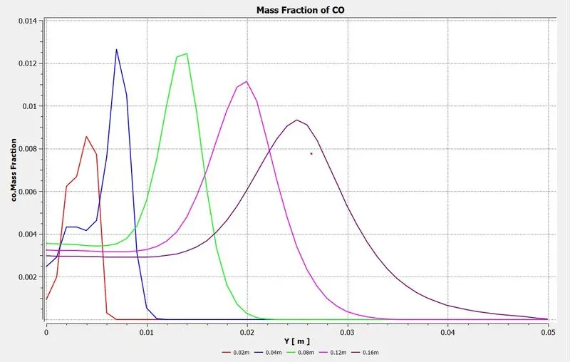
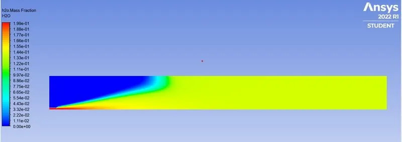
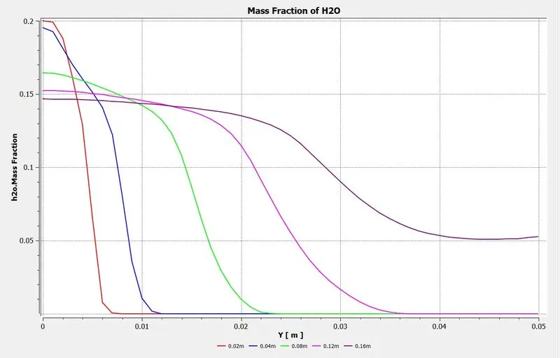
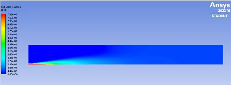
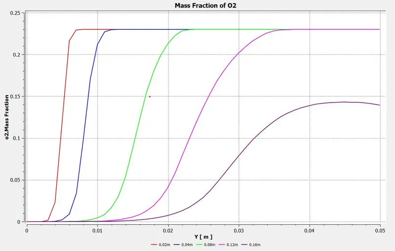
Aim: To perform simulation of combustion of natural gas methane and analysis of species present during the combustion reaction. also, observe the effect on the combustion due to the addition of water content with the fuel.
Introduction:
The emission of pollutants in the combustion process has an adverse effect on both the environment and combustion devices. The efficiency of combustion devices decreases due to pollutants which are by-products of the combustion process. Oxides of carbon, nitrogen, sulphur, unburnt fuel etc. are some of the pollutants that produce by the combustion of hydrocarbon fuel emissions of these pollutants in the environment lead to climate change. That’s why analysis of the formation of by-products during the combustion of fuels helps in finding the solution to the reduction of pollution.
Combustion is an exothermic reaction where the reductant such as fuel reacts with oxidants at high temperature producing enormous heat and oxidizes.
The generalized chemical equation for stoichiometric combustion of hydrocarbon with oxygen is:
`C_xH_y + zO_2 -> xCO_2 + y/2 H_2O`
Though the above equation is generalized, combustion is a more complicated reaction due to many intermediate reactions that take place during the combustion. The study of those reactions and the kinematics is an important part of the analysis.
With the help of computer simulation, we can model the combustion reaction using mathematical models for the analysis of the mass fraction of the compounds that are present during the combustion reaction.
Types of combustion simulation
Non-premixed combustion:
In this type of combustion, oxidizer and fuel enter the reaction zone as distinct streams.
Premixed combustion
The fuel and the oxidizer are premixed before the combustion
Partially Premixed
It is in between non-premixed and premixed where the fuel and oxidizer are mixed at a non-uniform reaction before combustion.
Procedure:
Workbench:
- Open ANSYS WORKBENCH. Drag and drop Fluent.
-Click on File and Save the Project as ‘Combustion_of_Natural_Gas’.
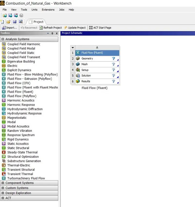
Geometry:
-Open SpaceClaim and import the downloaded geometry.
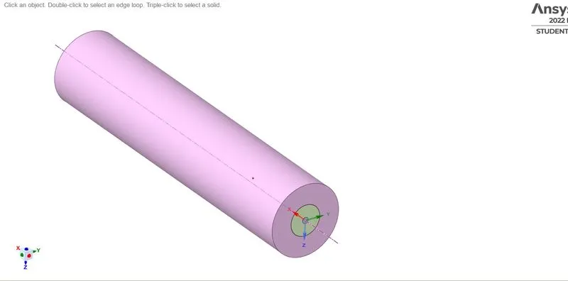
-To reduce the computational effort for this simulation, split the 3D model in one-fourth.
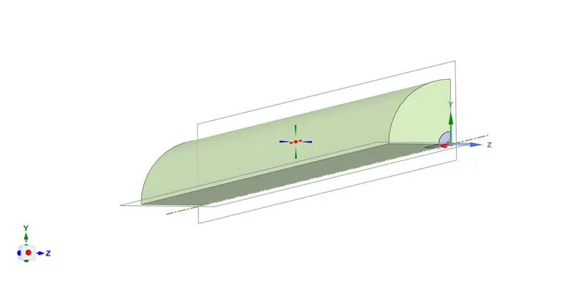
-Copy and paste the 2D plane normal to Z-axis in new window
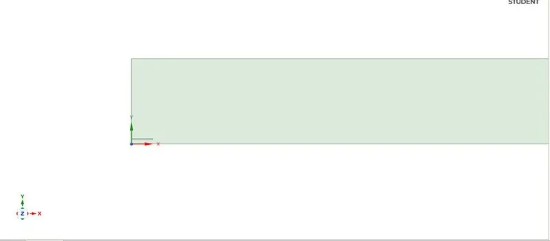
-Click on File and Save the Project.
Meshing:
-Open Meshing and specify the names for edges (boundaries).
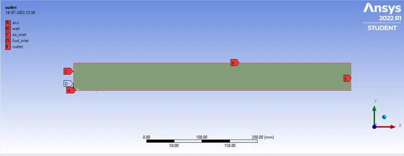
-Generate the mesh with element size of 1mm.
-Opt for capture proximity with 5 cells gaps.
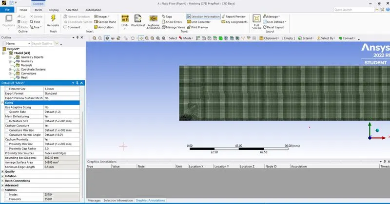
-Click on File and Save the Project.
Fluent Setup:
-Open the Setup (Fluent) and set up the following condition
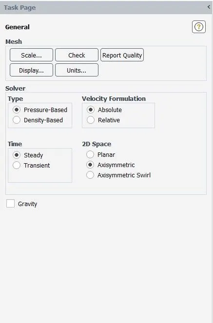
-Check the 2D space axisymmetric model box as we are performing axisymmetric analysis.
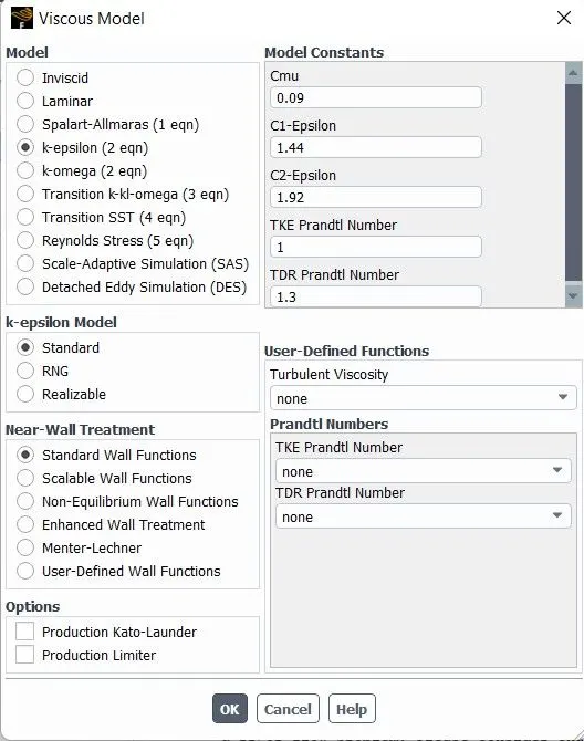
-Choose a k-epsilon viscous model with standard wall function as combustion reaction is turbulent.
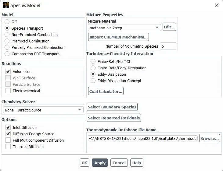
-Choose Species Transport model for Species model and mixture material s methane-air-2step. Check the Volumetric Reaction box. Choose the Eddy dissipation model for chemical interaction.
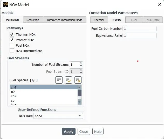
-For the NOx model, check Thermal NOx and Prompt NOx box. Specify methane as the primary fuel.
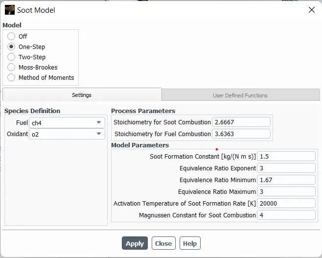
-For Soot Model, choose One step model with methane as fuel and oxygen as oxidant.
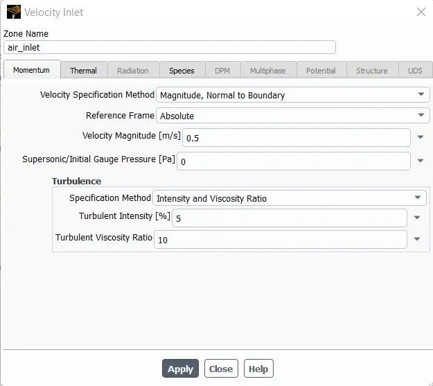
-Boundary conditions for
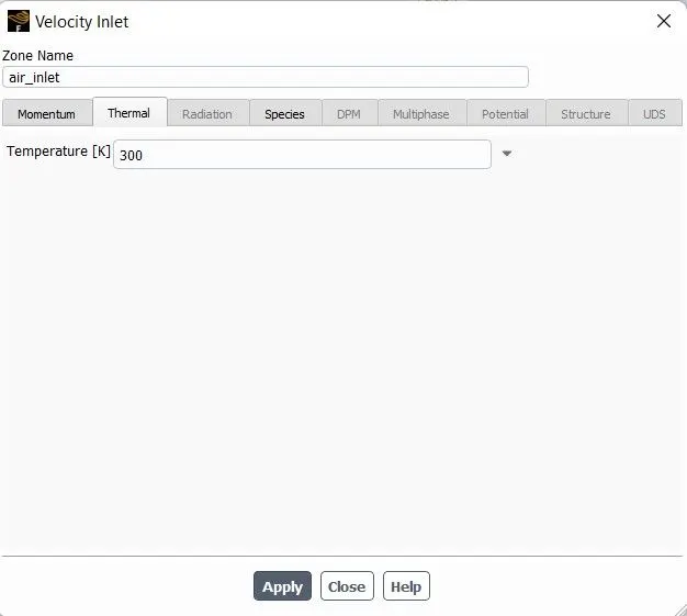
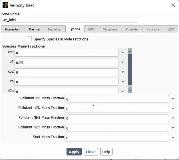
- Air inlet: Velocity- 0.5 m/s
Thermal – 300 K
Species- Oxygen to 0.23 (mass fraction) and rest of species to 0.
 |
 |
 |
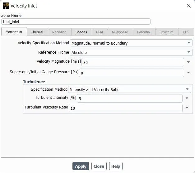
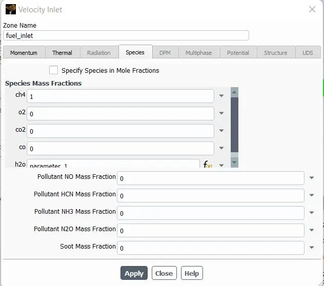
- Fuel inlet: Velocity- 80 m/s
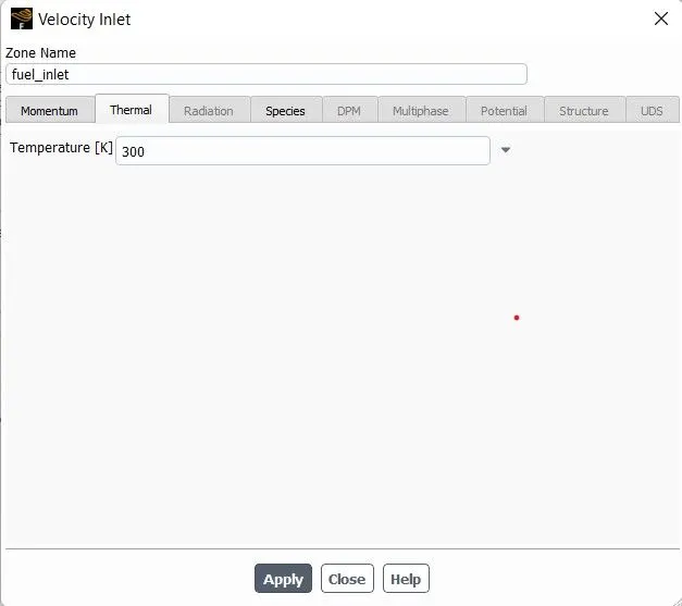
Thermal: 300 K
Species: Methane to 1.
For the second case where we add water with the fuel up to 30% mass fraction for methane and water is specified.
In that case, for 5% of water, the mass fraction for methane is 0.95 and water is 0.05.
 |
 |
|
-Initialize the solution and run the calculation.
Results:
Case 1:
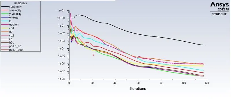
Residual Plot
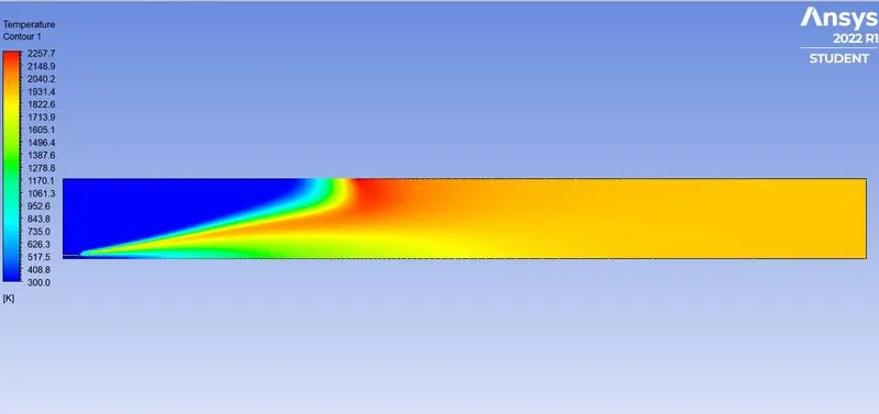
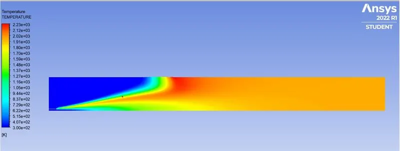
Temperature Contour
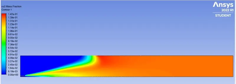
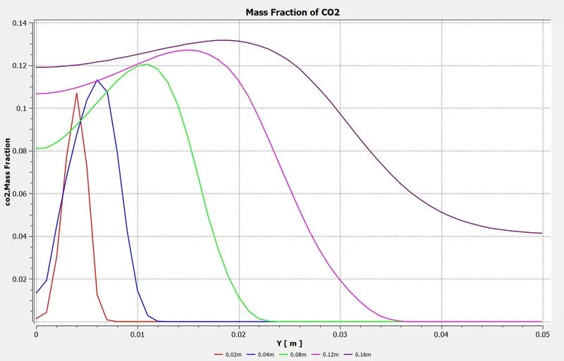
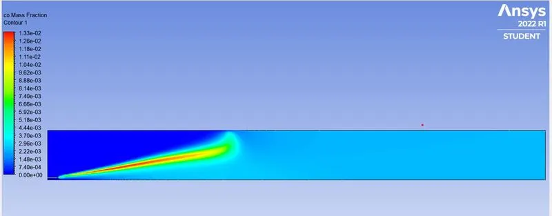
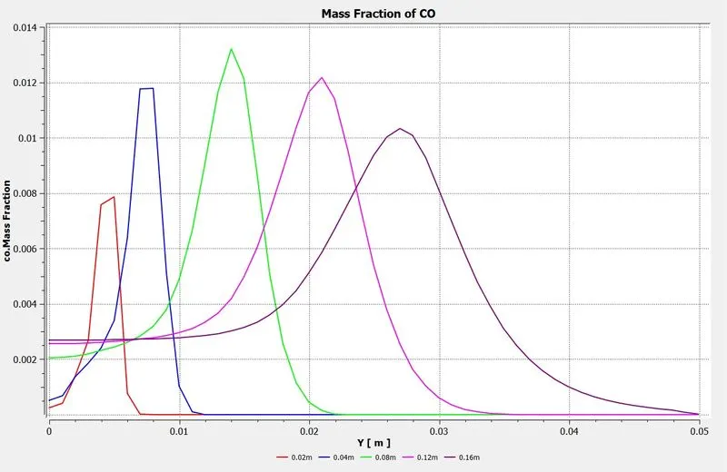
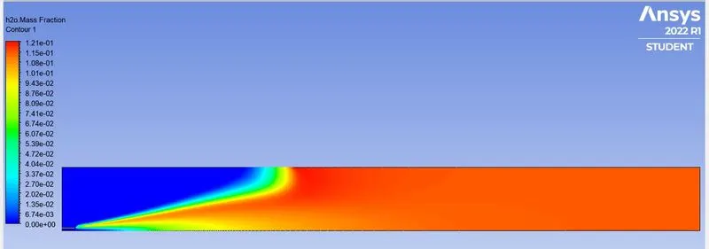
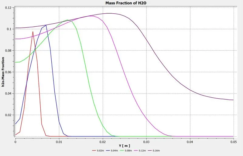
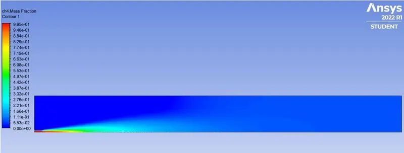
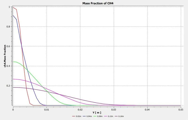
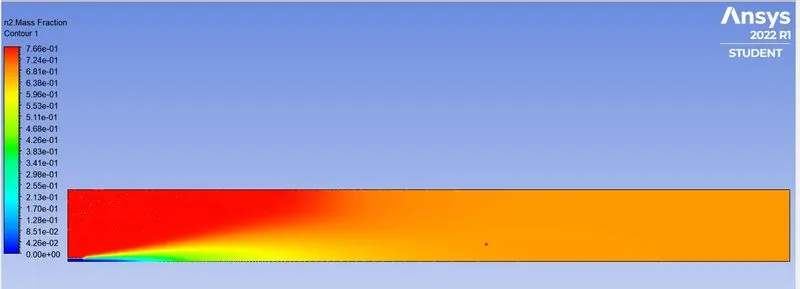
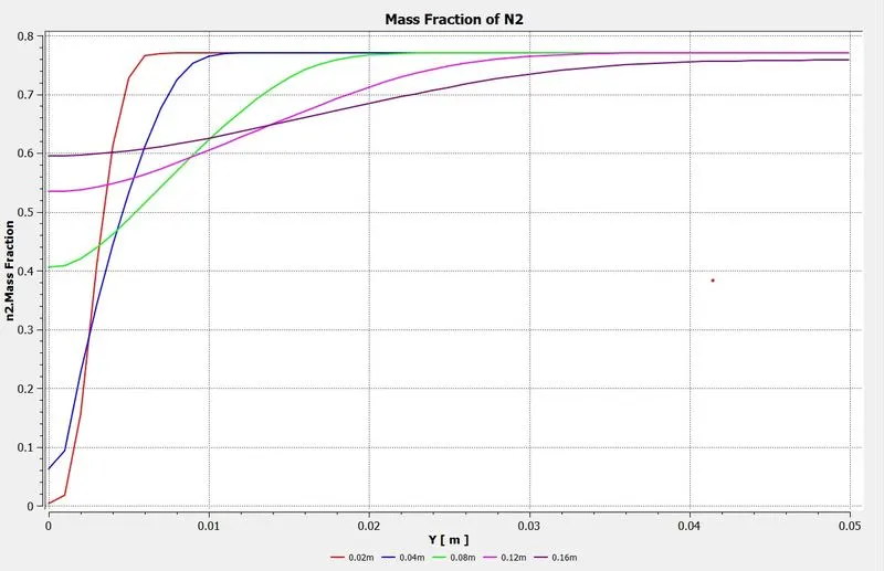
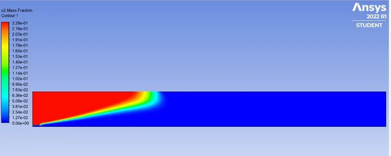
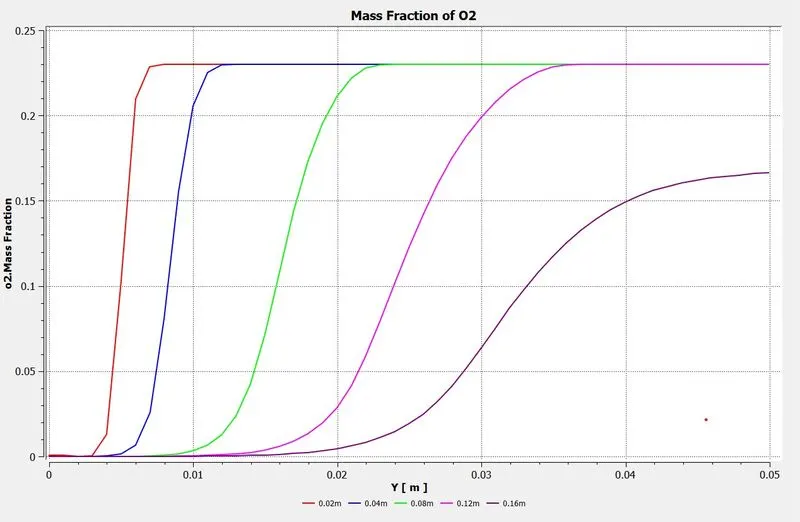
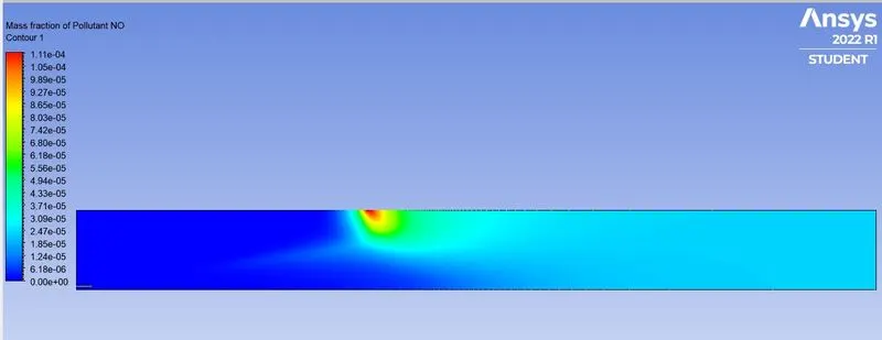
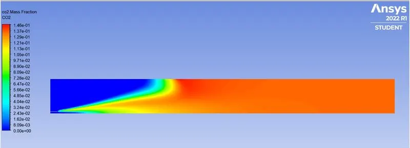
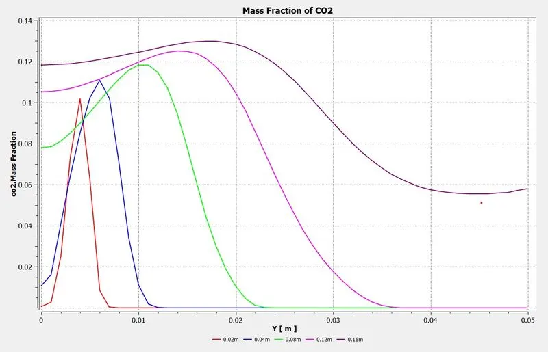
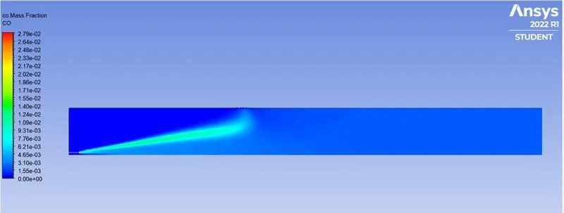
Plots for Mass Fraction
|
Emissions |
Contour |
Line Plot |
|
CO2 |
 |
 |
|
CO |
 |
 |
|
H2O |
 |
 |
|
CH4 |
 |
 |
|
N2 |
 |
 |
|
O2 |
 |
 |
|
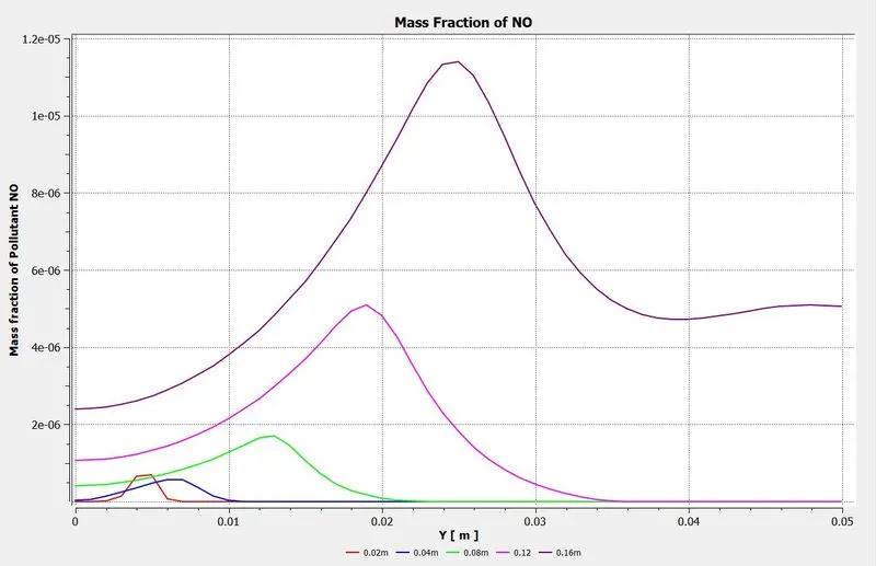
NOx |
 |
 |
|
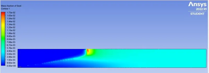
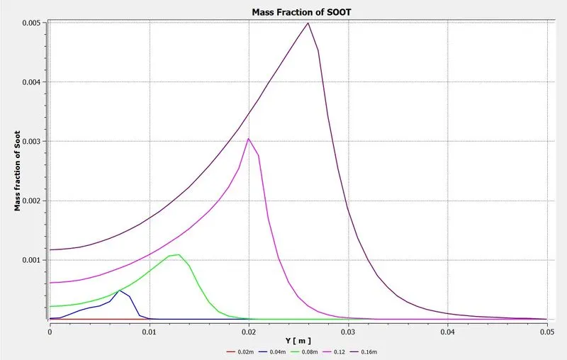
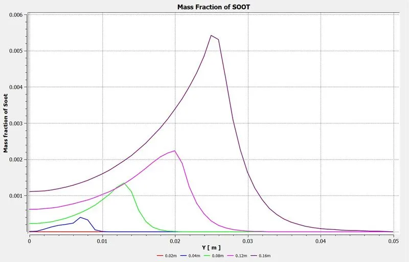
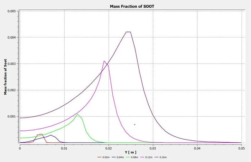
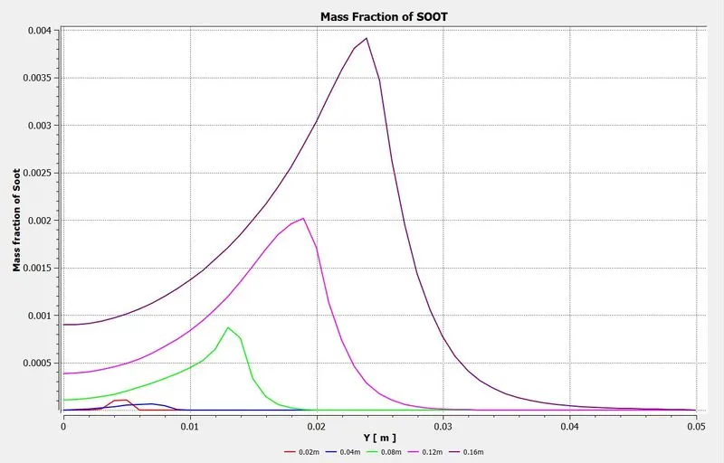
SOOT |
 |
 |
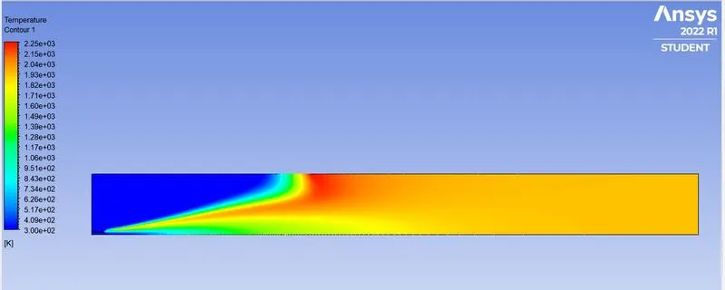
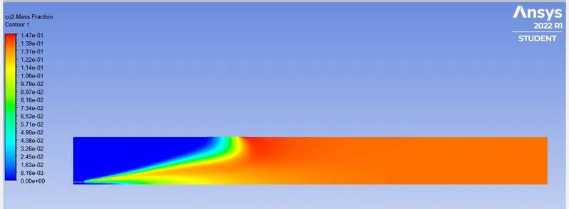
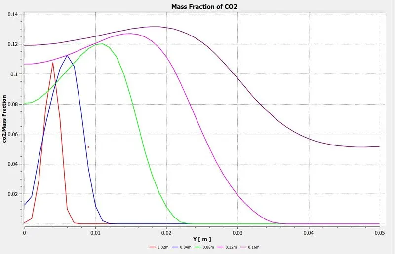
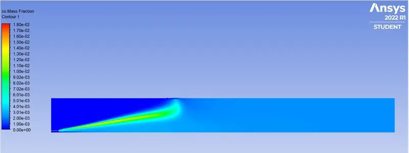
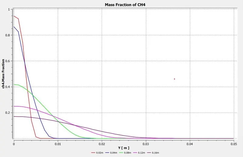
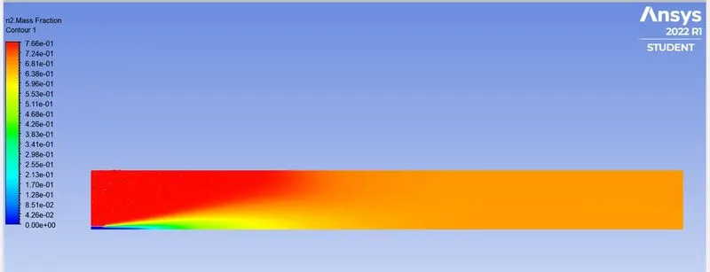
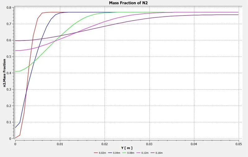
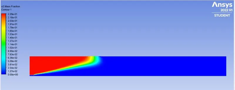
Case 2A: 5% WATER
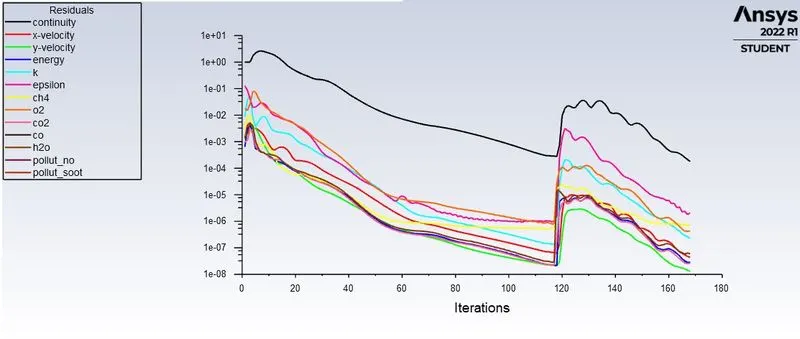
Residual Plot
Temperature Contour
|
Emissions |
Contour |
Line Plot |
|
CO2 |
 |
 |
|
CO |
 |
 |
|
H2O |
 |
 |
|
CH4 |
 |
 |
|
N2 |
 |
 |
|
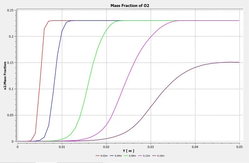
O2 |
 |
 |
|
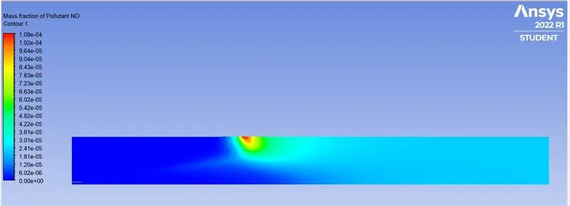
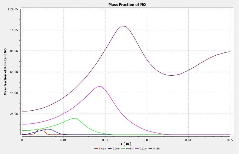
NOx |
 |
 |
|
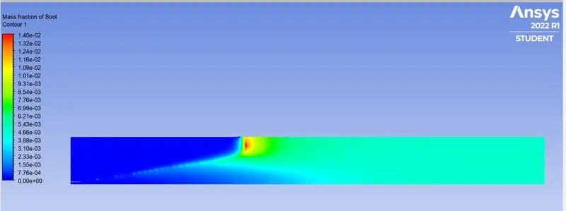
SOOT |
 |
 |
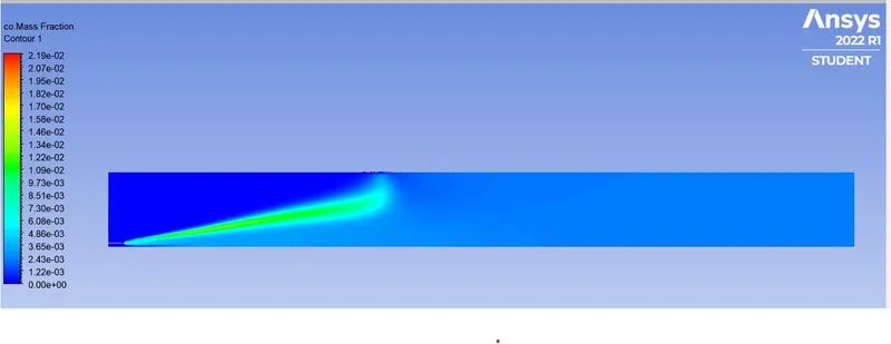
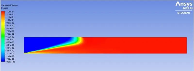
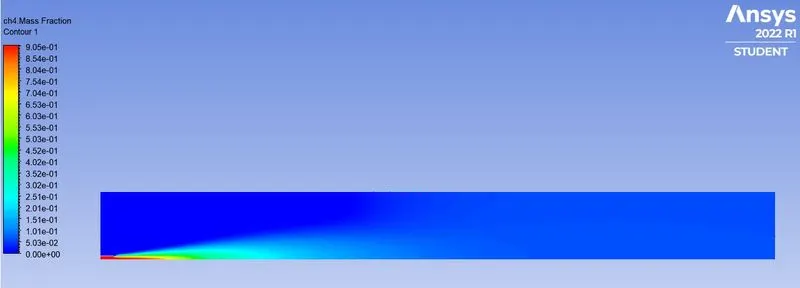
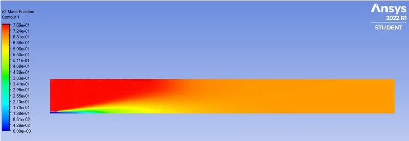
Case 2B: 10% WATER
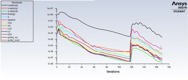
Residual Plot
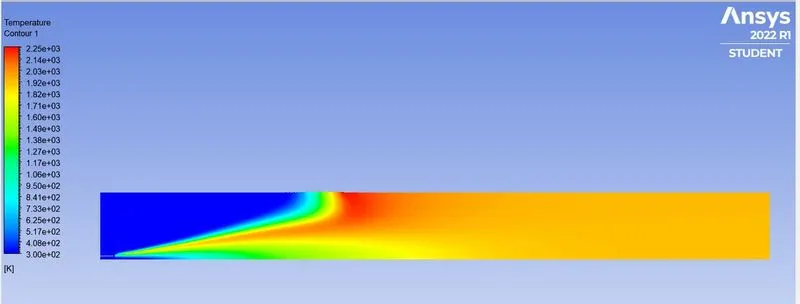
Temperature Contour
|
Emissions |
Contour |
Line Plot |
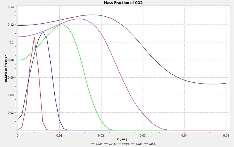
|
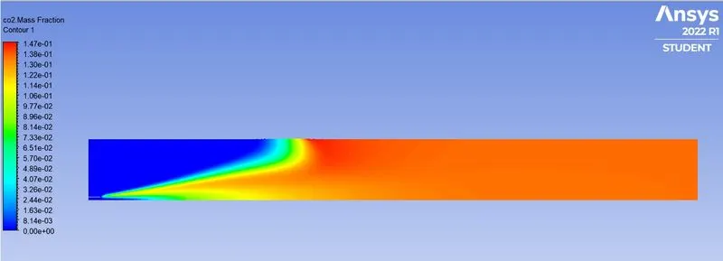
CO2 |
 |
|
|
CO |
 |
|
|
H2O |
 |
|
|
CH4 |
 |
|
|
N2 |
 |
|
|
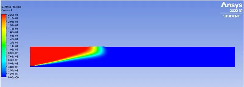
O2 |
 |
|
|
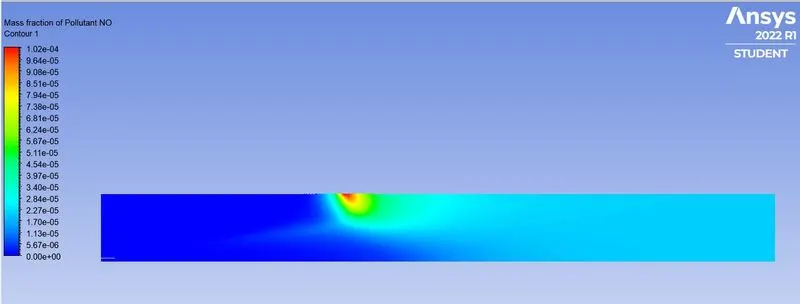
NOx |
 |
|
|
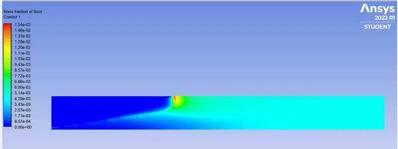
SOOT |
 |
|
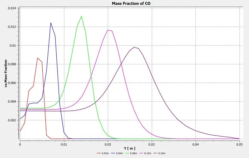
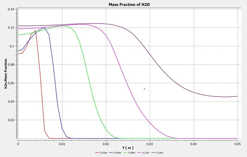
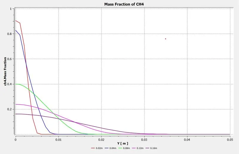
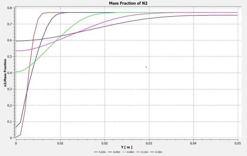
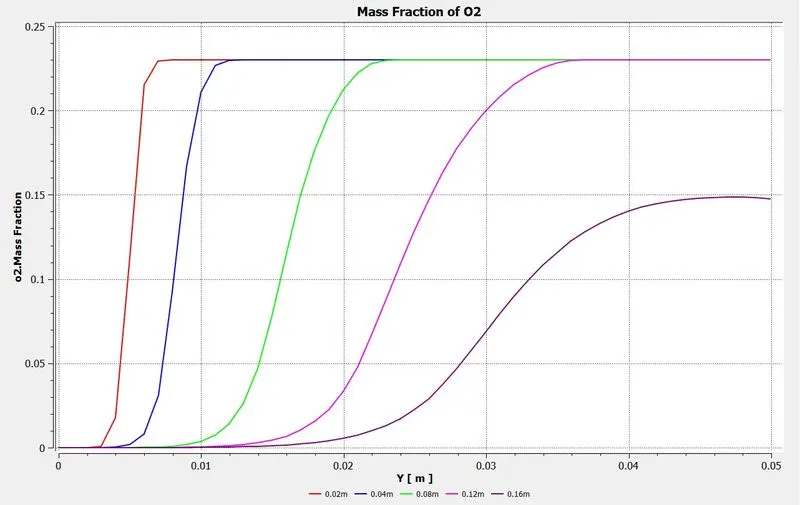
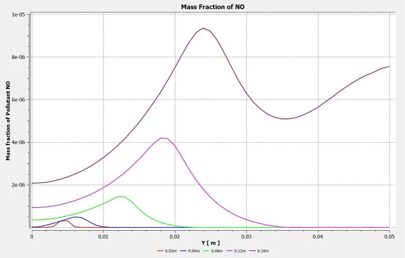
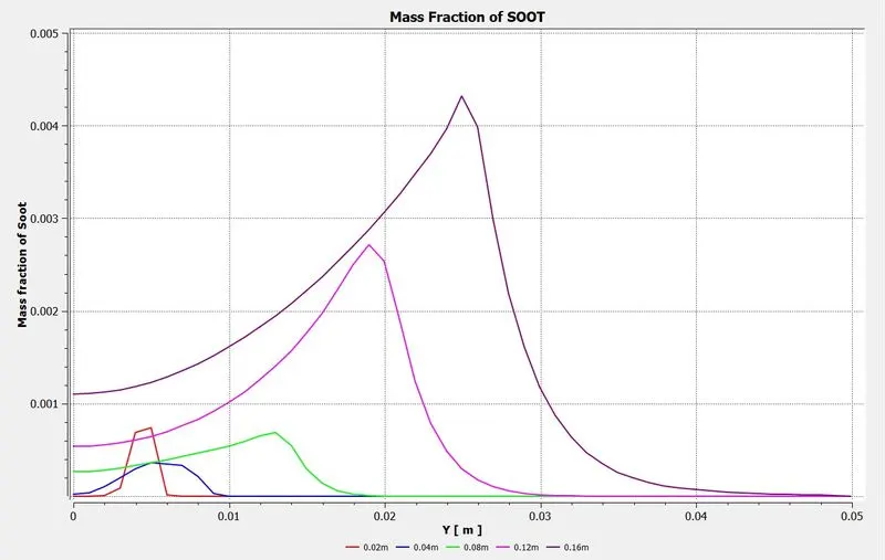
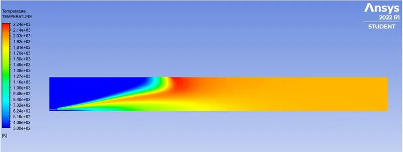
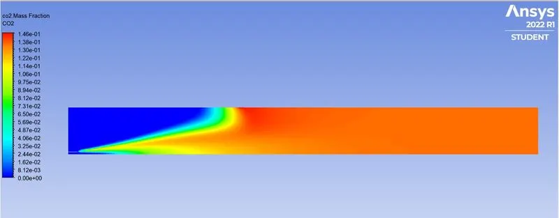
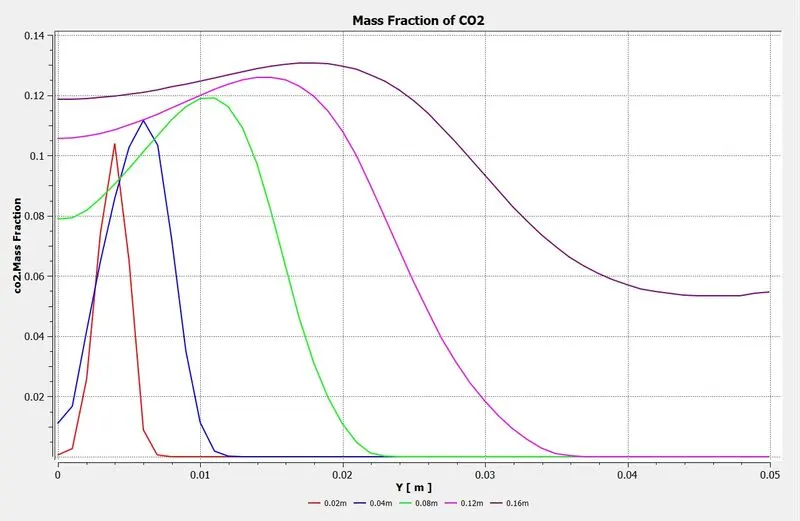
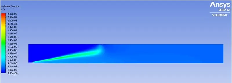
Case 2C: 15% WATER
Residual Plot
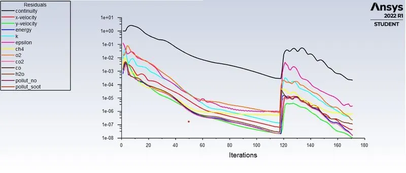
Temperature Contour
|
Emissions |
Contour |
Line Plot |
|
CO2 |
 |
 |
|
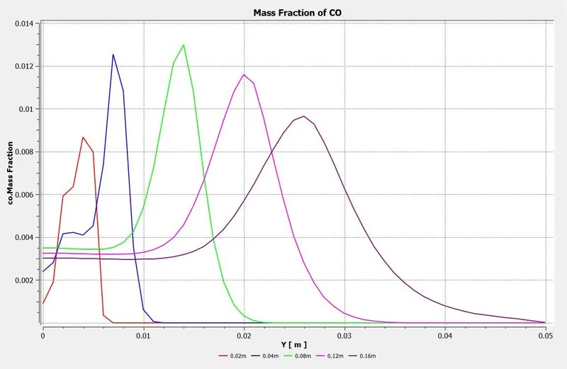
CO |
 |
 |
|
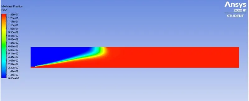
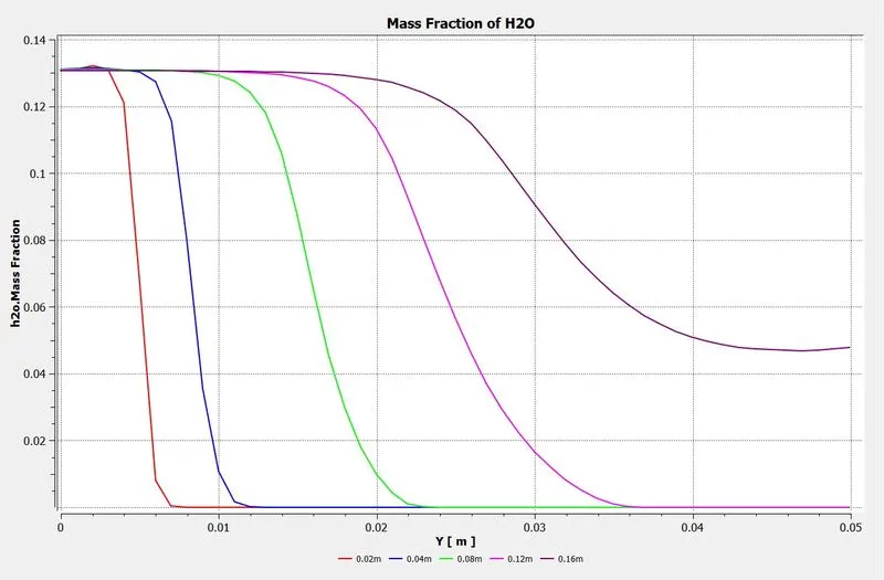
H2O |
 |
 |
|
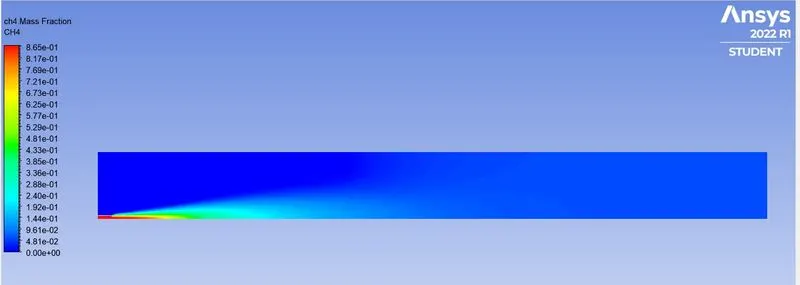
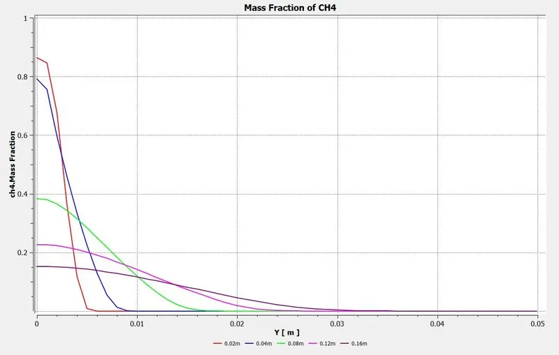
CH4 |
 |
 |
|
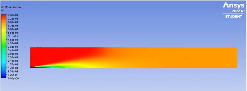
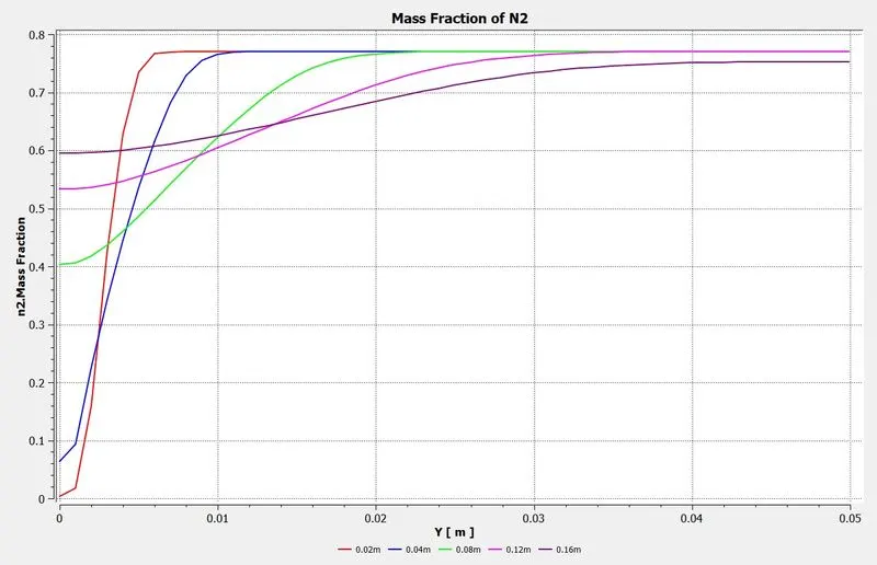
N2 |
 |
 |
|
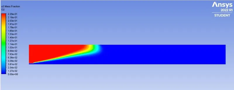
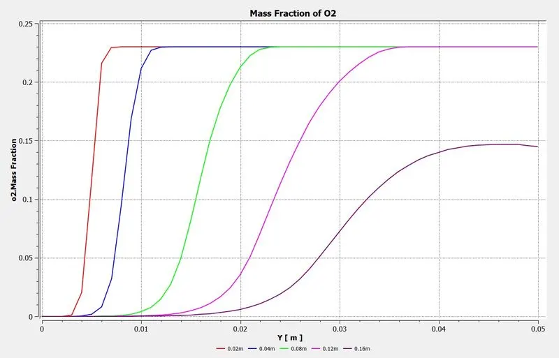
O2 |
 |
 |
|
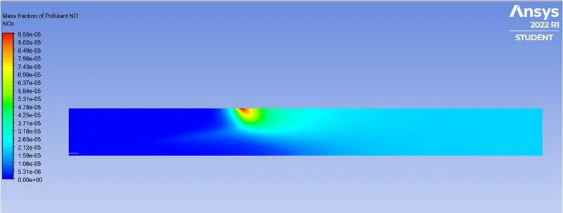
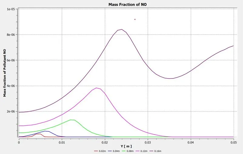
NOx |
 |
 |
|
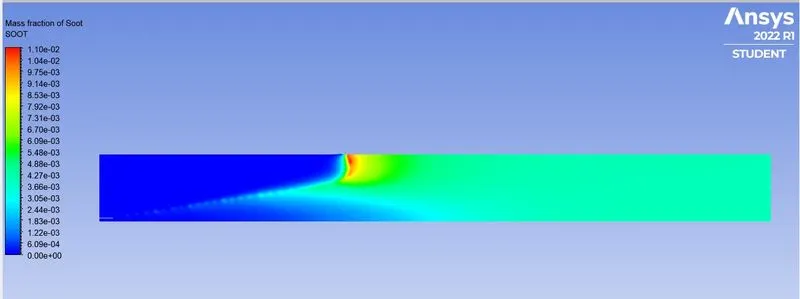
SOOT |
 |
 |
Case 2D: 20% WATER
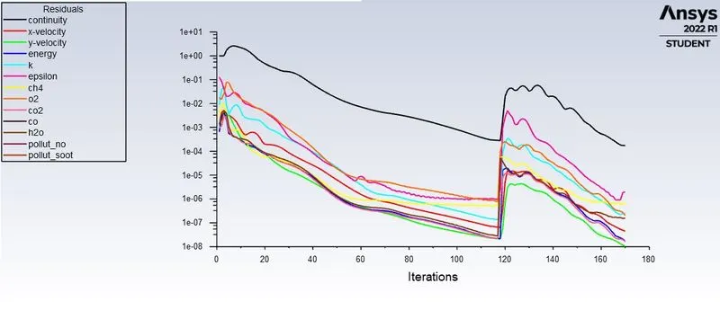
Residual Plot
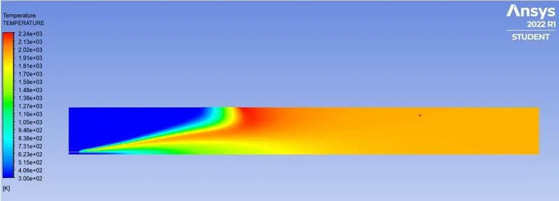
Temperature Contour
|
Emissions |
Contour |
Line Plot |
|
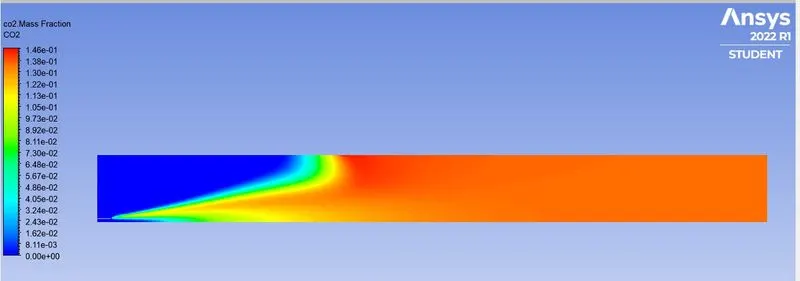
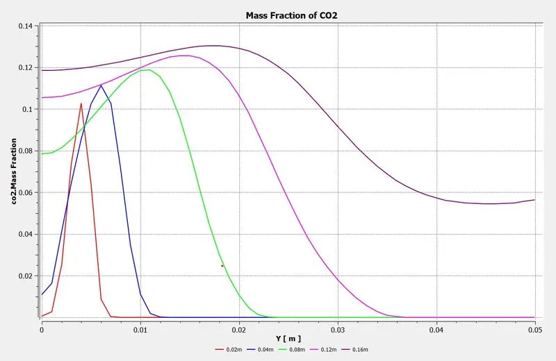
CO2 |
 |
 |
|
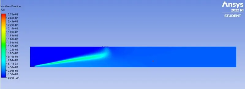
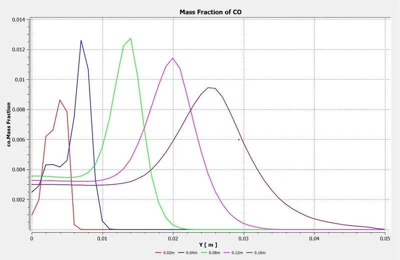
CO |
 |
 |
|
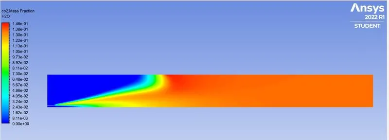
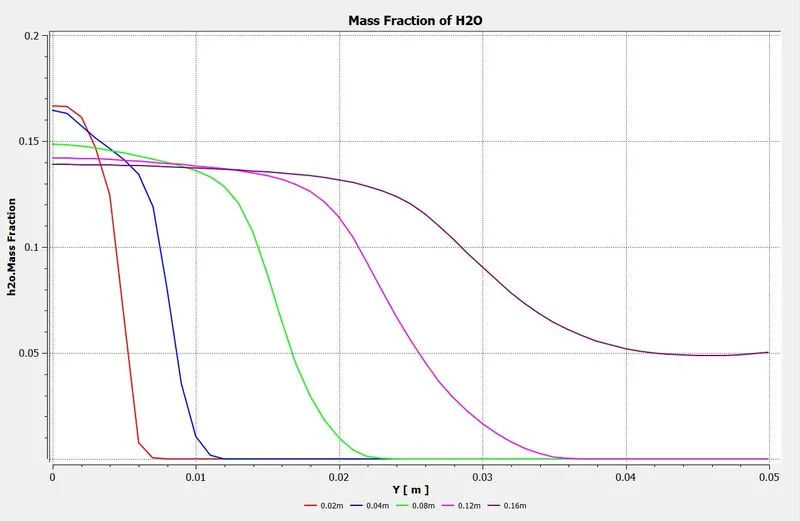
H2O |
 |
 |
|
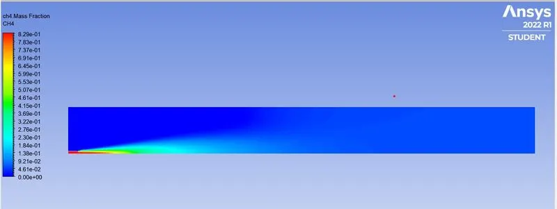
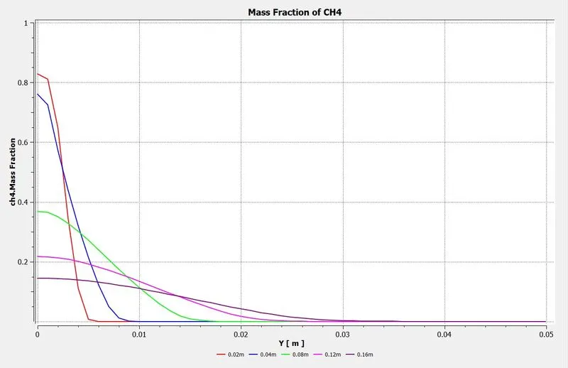
CH4 |
 |
 |
|
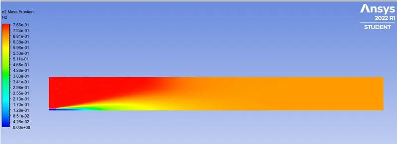
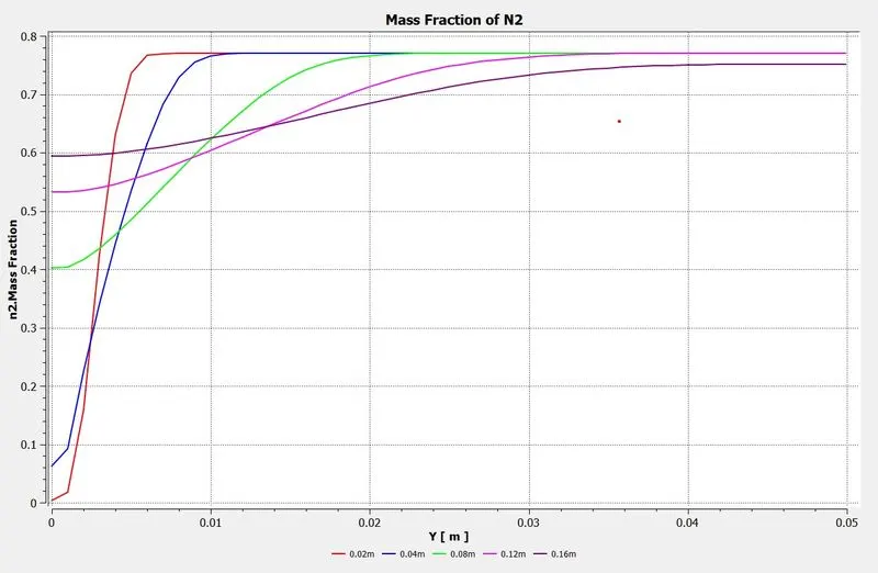
N2 |
 |
 |
|
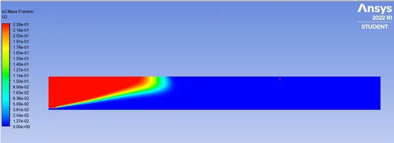
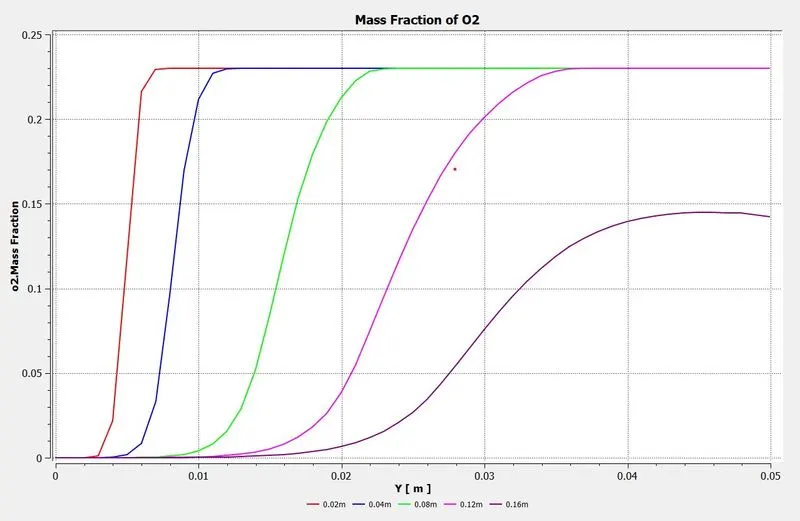
O2 |
 |
 |
|
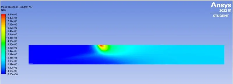
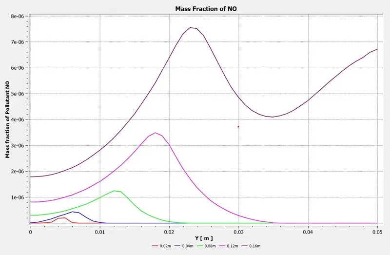
NOx |
 |
 |
|
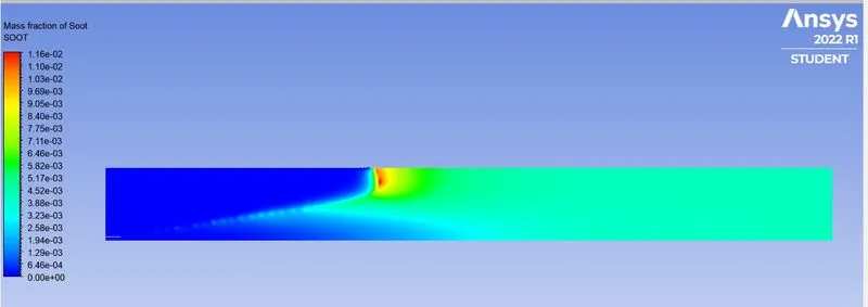
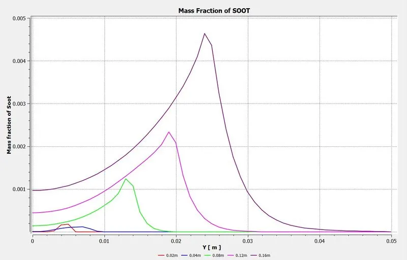
SOOT |
 |
 |
Case 2E: 25% WATER
Residual Plot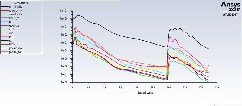
Temperature Contour
|
Emissions |
Contour |
Line Plot |
|
CO2 |
 |
 |
|
CO |
 |
 |
|
H2O |
 |
 |
|
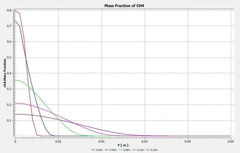
CH4 |
 |
 |
|
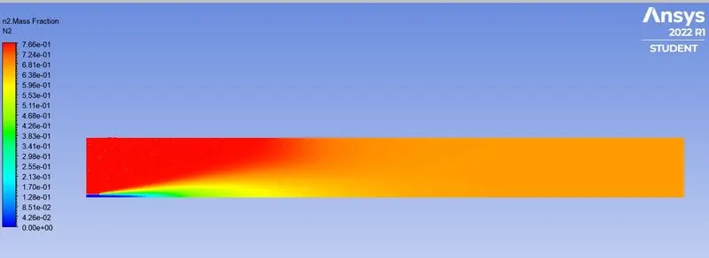
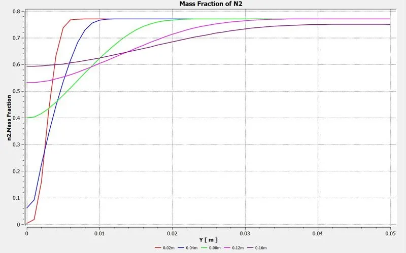
N2 |
 |
 |
|
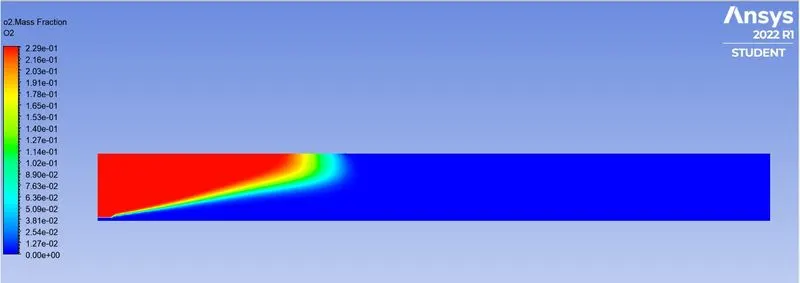
O2 |
 |
 |
|
NOx |
 |
 |
|
SOOT |
 |
 |
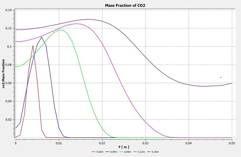
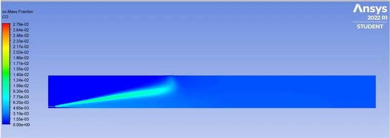
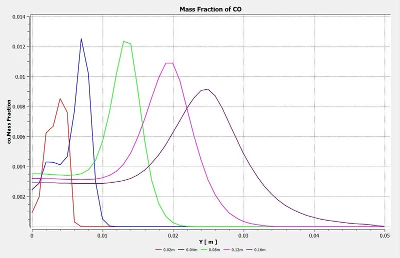
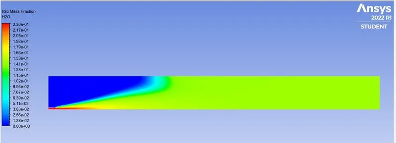
Case 2F: 30% WATER
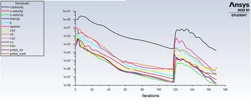
Residual Plot
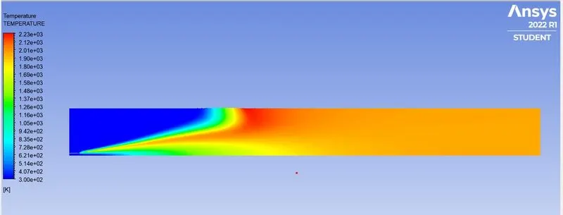
Temperature Contour
|
Emissions |
Contour |
Line Plot |
|
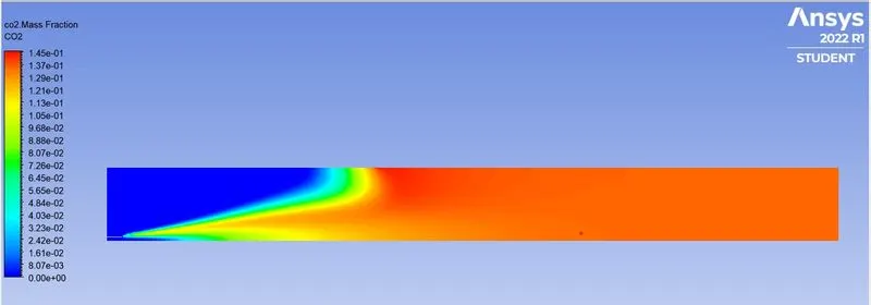
CO2 |
 |
 |
|
CO |
 |
 |
|
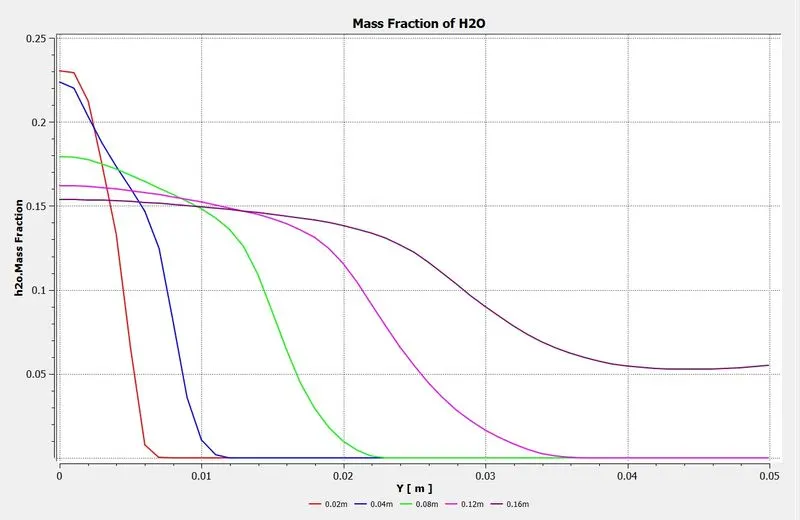
H2O |
 |
 |
|
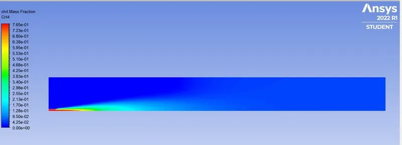
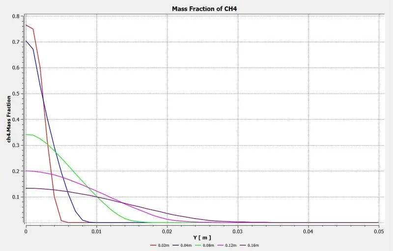
CH4 |
 |
 |
|
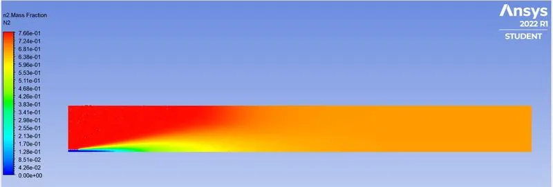
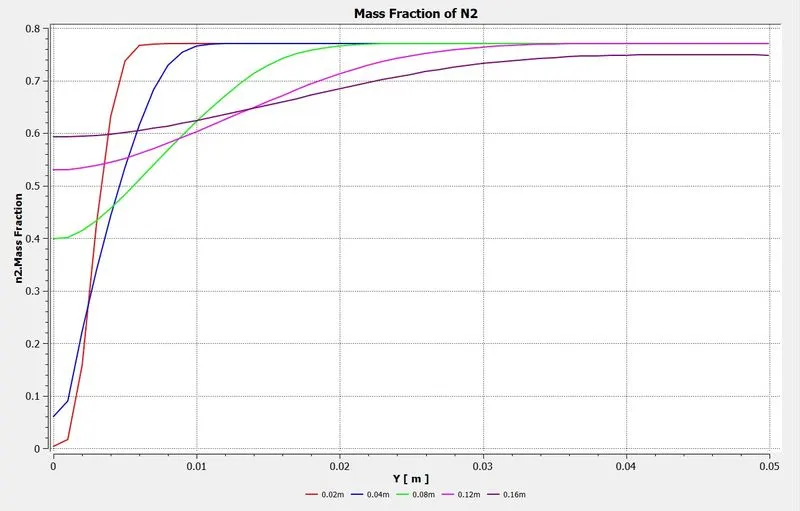
N2 |
 |
 |
|
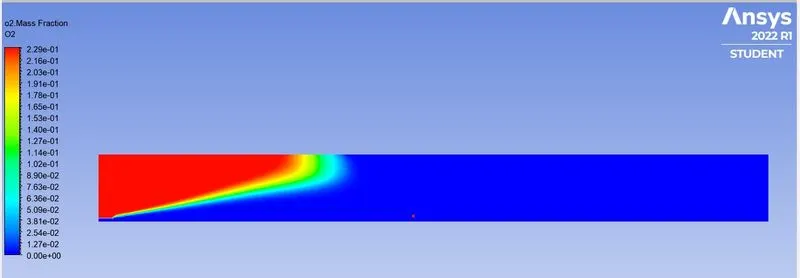
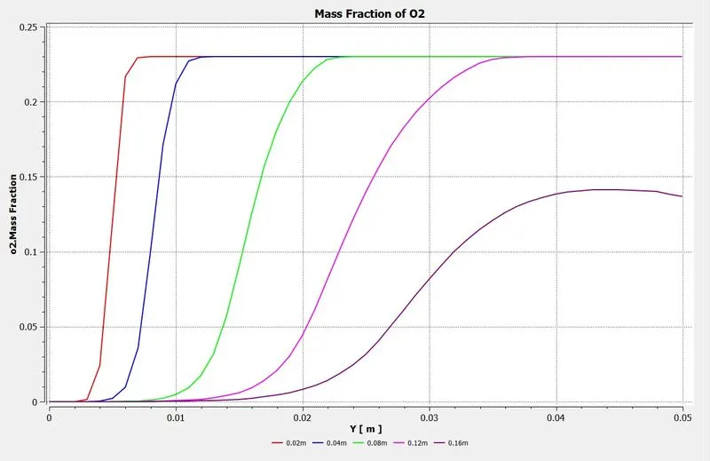
O2 |
 |
 |
|
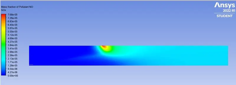
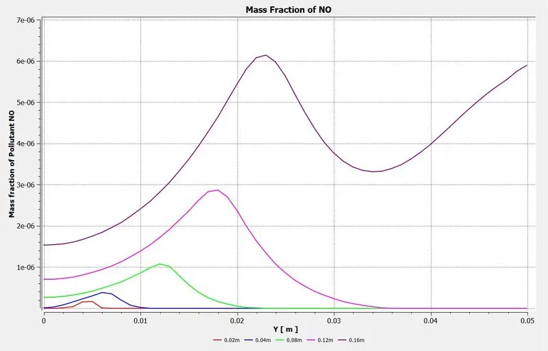
NOx |
 |
 |
|
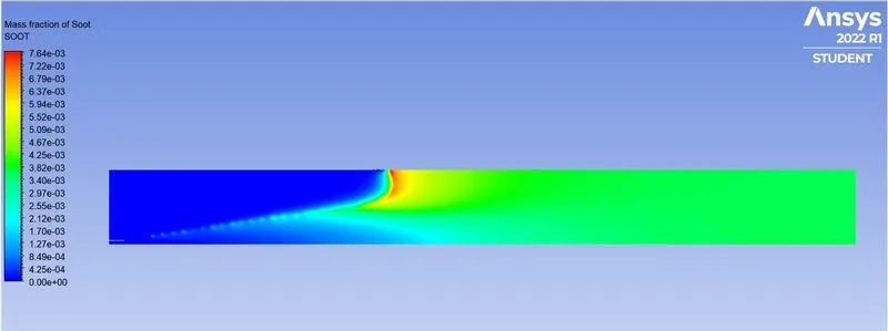
SOOT |
 |
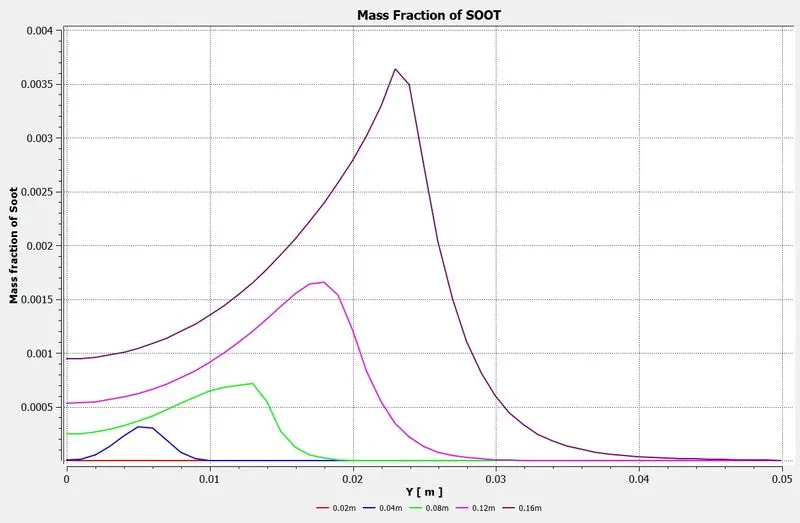 |
Conclusion:
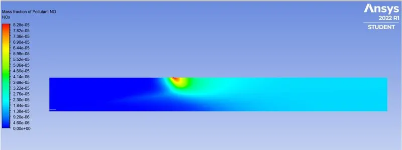
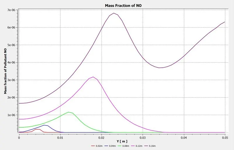
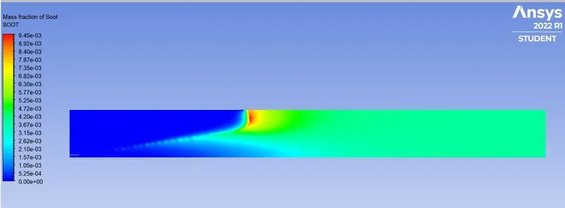
From the above plots, it is observed that the NOx and soot formation is reduced with an increase in the water content in the methane. The temperature decrease leads to a delay in combustion causing an efficient mixture of fuel and air. With the proper mixture of fuel and air and a decrease in temperature, formation nitrogen oxides decreases.