Week 1: Channel flow simulation using CONVERGE CFD
Channel flow simulation using CONVERGE CFD
AIM: To simulate the flow through the channel using CONVERGE CFD.
OBJECTIVE:
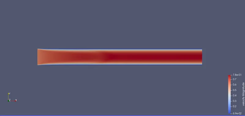
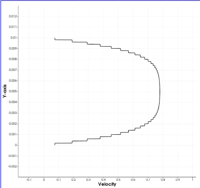
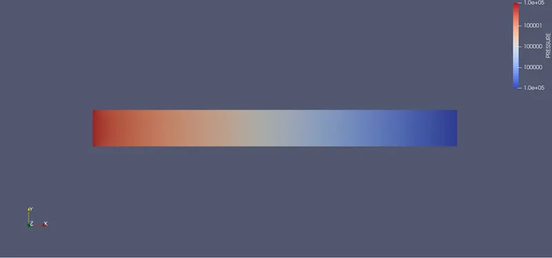
The objective of the present project is to set up the simulation of flow through the channel for 3 different meshes in the Converge and create contour velocity and pressure contour plots for three different meshes.
THEORY:
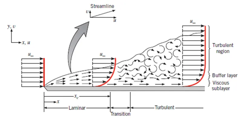
The boundary layer in fluid dynamics refers to the layer of fluid that is near the surface boundary where the effect of viscosity is evident and significant.
The nature of the boundary layer formation depends on the Reynolds number. The fluid flow is either laminar or turbulent depending on the Reynolds number. Reynolds number is the ratio of inertial forces to viscous forces. The flow regime for Reynolds number below 2000 is laminar flow, between 2000 to 4000 is transition flow and above 4000 is turbulent flow.
For the laminar flow, the boundary layer is laminar and the streamwise velocity is uniformly changing as moving away from the wall. Whereas for turbulent flow, the boundary layer is turbulent and the streamwise velocity is unsteady with swirling flow.
PROCEDURE:
Pre-Processing:
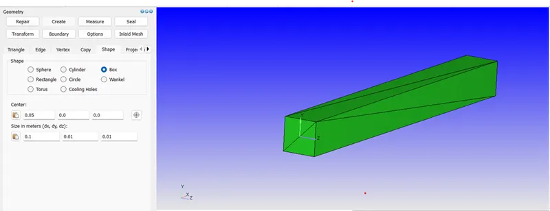
-Open Converge and create the required geometry using the Create tool.
-Select the Shape option and choose the Box option. Specify the centre as (0.05,0.0,0.0) m and size as (0.1,0.01,0.01) m.
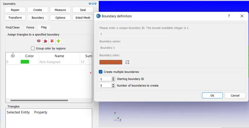
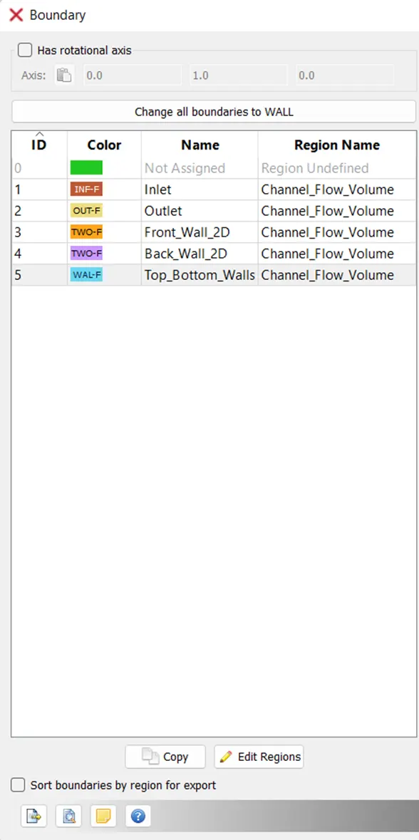
-Specify the boundaries using The Boundary option and click on the “Plus” symbol to create the boundaries. In the Boundary Definition tb, check the Create multiple boundaries option and specify the Number of boundaries to create as 5. Click on ok
-Rename the boundaries by right-clicking on the boundary name. To assign the boundary, click on the boundary name and select the corresponding boundary surface. Click on Apply to proceed.
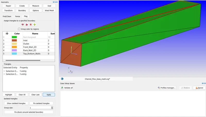
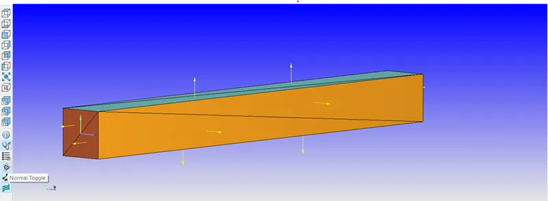
-To view the normal of the surfaces, click on the Normal Toggle option. As observed, the normal is pointing outwards. But the flow is within the boundaries so, the normal should be pointing inwards.
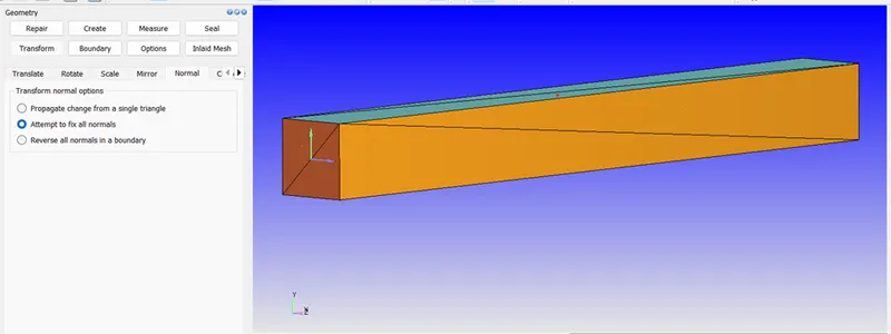
-To transform the normal, click on the Transform option and select the Normal option. Select the attempt to fix all normal options and click on Apply to proceed.
Simulation Set-up and Meshing:
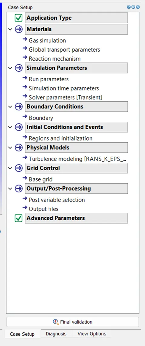
-Click on the Begin Case Setup in the Case setup dock.
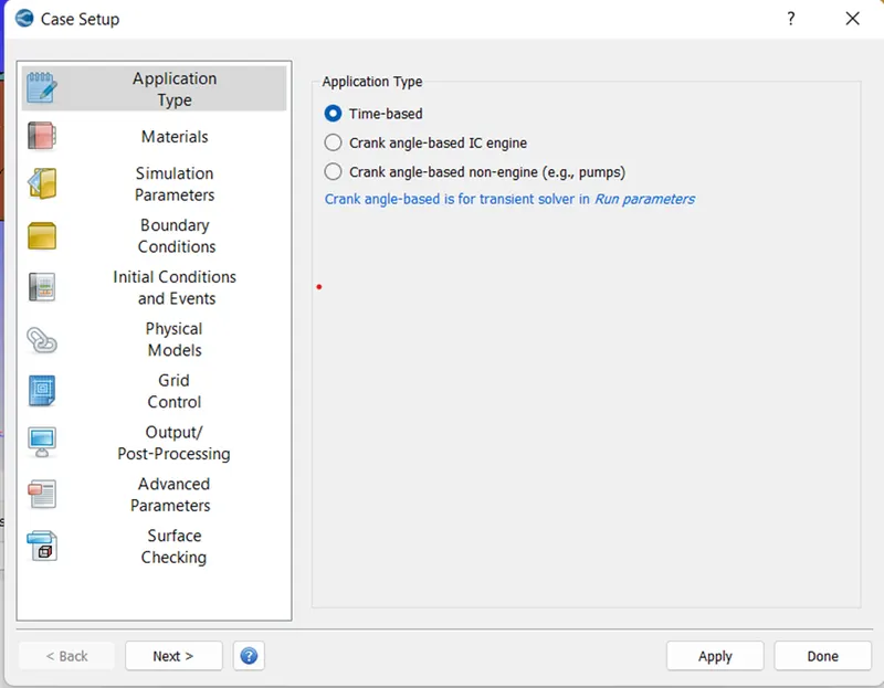
-To perform the steady-state simulation, select the Time-Based in the Application type. Click on apply and Done.
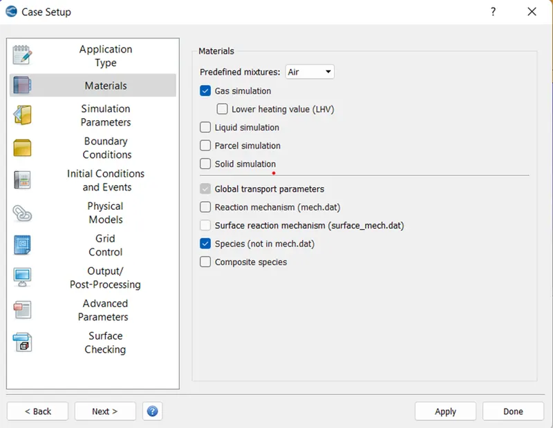
-For the Material, select ‘Air’ as Pre-Defined mixtures with the check on Gas simulation and Species.
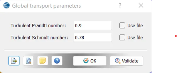
-For the Global transport parameter, specify the Turbulent Prandtl number as 0.9 and the Turbulent Schmidt number as 0.78. Click on Ok and Validate
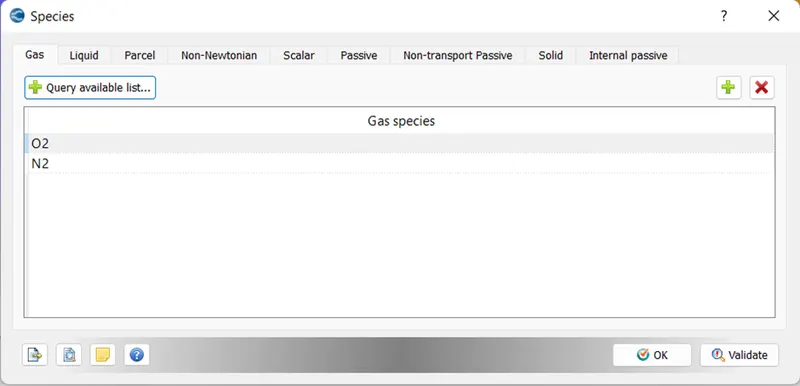
-For the Species, click on the ‘Plus’ symbol to add new species. Since this simulation is a gas simulation, we will add N2 and O2 in the Gas tab.
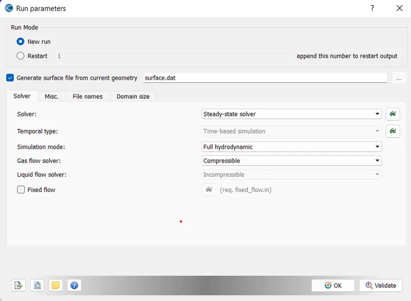
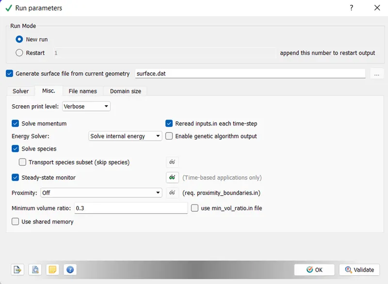
-For the Run Parameters, in the Solver tab specify the Solver as Steady-State Solver, Simulation mode as Full-hydrodynamic, and Gas flow solver as Compressible.
-In the Misc. tab, check the Steady-State monitor and uncheck the Use shared memory.
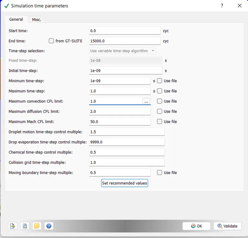
-For the Simulation Time Parameter, specify the details as shown in the following image.
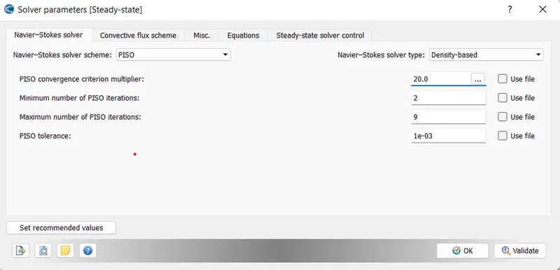
-For the Solver Parameter [Steady-State], use the Density-Based Navier-Stokes solver type. In the Equations tab, make sure that the precondition is set to none for all the equations.
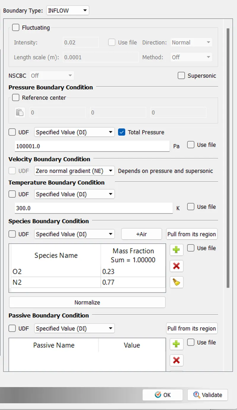
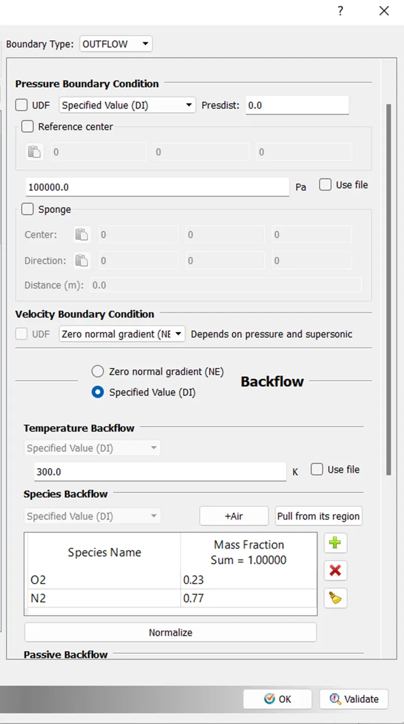
-Boundary Conditions are shown in the image
|
Inlet |
Outlet |
 |
 |
-Top and Bottom Wall:
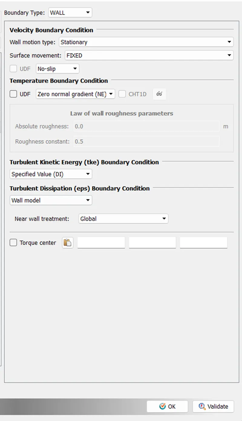
-Front and Back Walls:

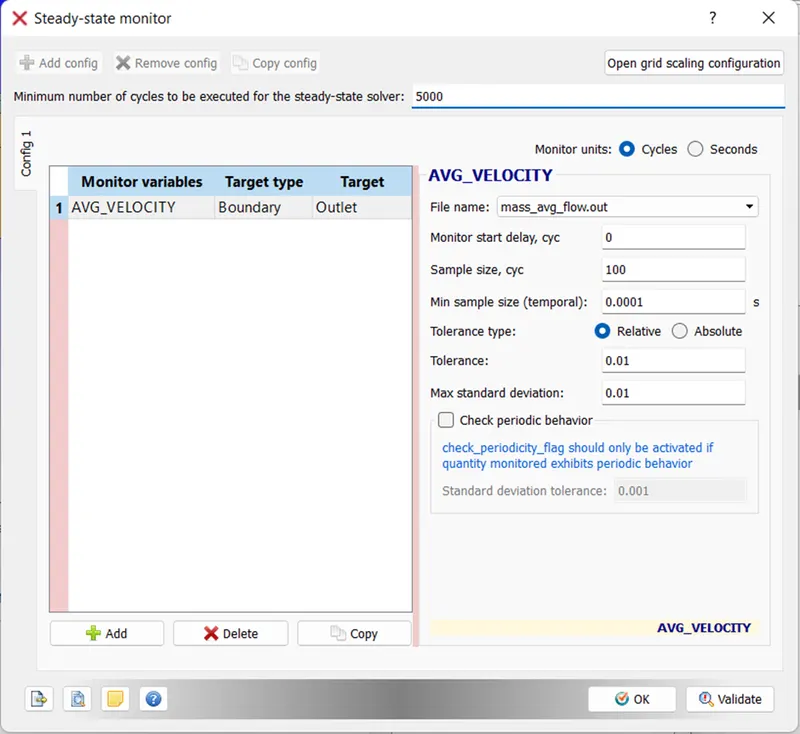
-Steady-State monitor helps in observing the data obtain from simulation. Create a steady-state monitor for Avg. velocity. A velocity monitor is a setup with tolerance to observe the convergence of the result.
-In the Region and Initialization tab, Create the region/volume where the fluid will flow. Specify mass fraction for O2 as 0.77 and N2 as 0.23.
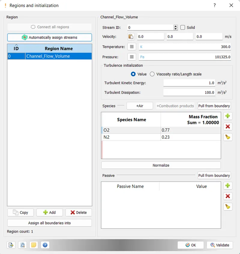
-Assign this region to all the boundaries.
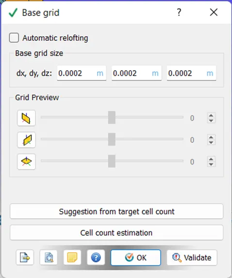
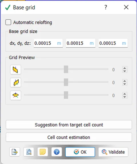
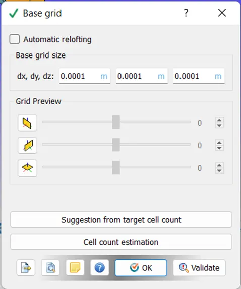
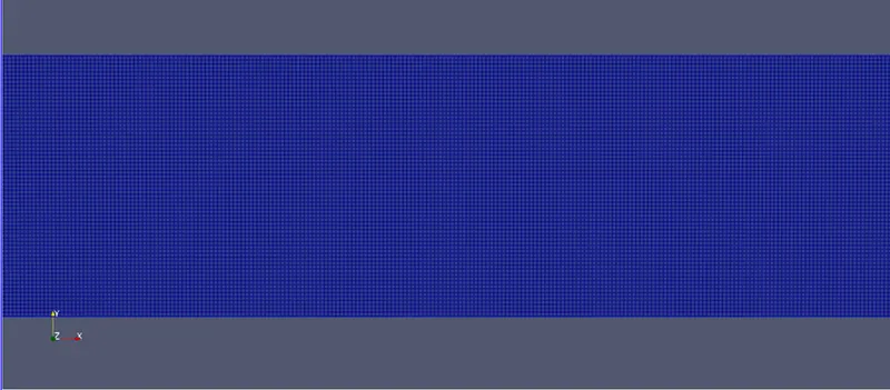
-Setup the mesh with 3 different grid sizes as mentioned below
- dx = 2e-4m, dy = 2e-4m, dz = 2e-4m
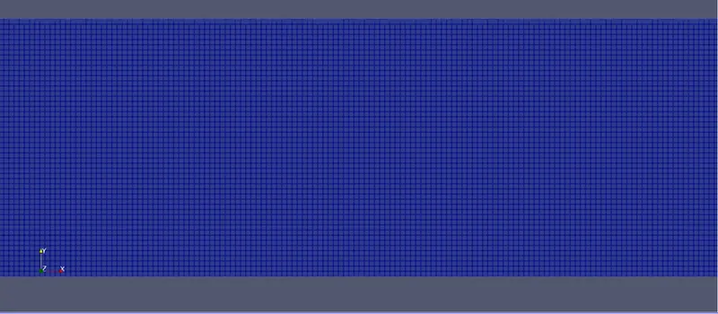
- dx = 1.5e-4m, dy = 1.5e-4m, dz = 1.5e-4m
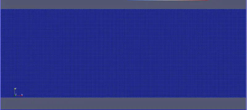
- dx = 1.0e-4m, dy = 1.0e-4m, dz = 1.0e-4m
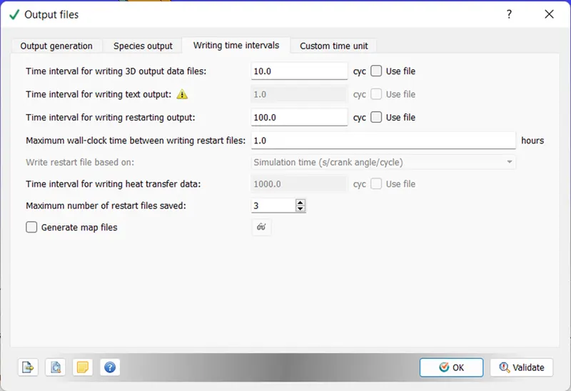
-In the Output file tab, specify the time interval for writing 3D output data files for 10 cycles. After 10 cycles it will create one 3D output file.
-The time interval for writing restarting output is specified as 100 cycles. If the simulation stops unexpectedly, it will help to restart the simulation in the last count of 100 cycles.
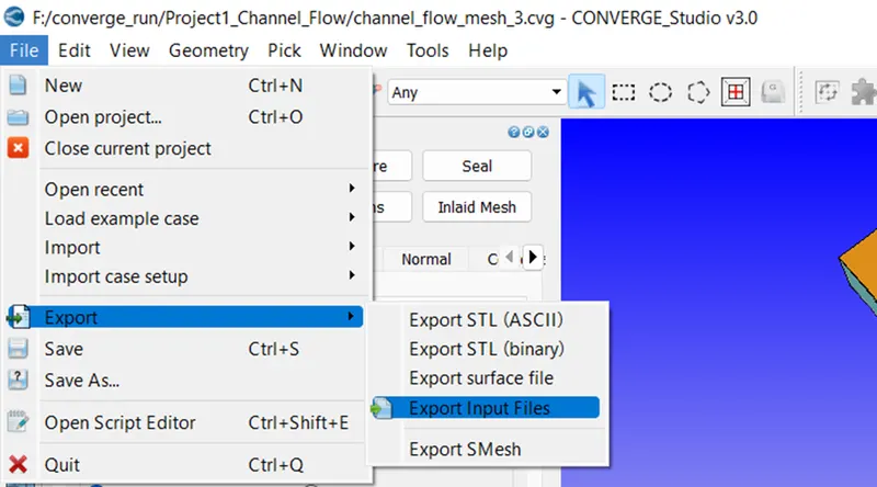
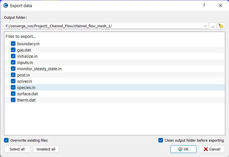
-After completing the simulation setup, export the input file to the desired folder. Click on the File then on Export. Select the Export Input Files option. Select the folder to export the input files and click on OK to complete the process.
Run the Simulation:
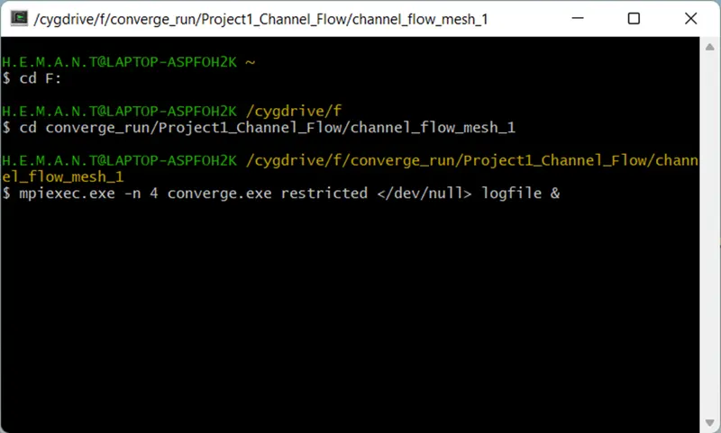
-To run the simulation, open the Cygwin terminal and open the folder which contains input files. Execute the command “mpiexec.exe -n 4 converge.exe restricted </dev/null> logfile &”. Before executing the command, paste the ‘mpiexec.exe’ and ‘converge.exe’ executables files into the input file’s folder.
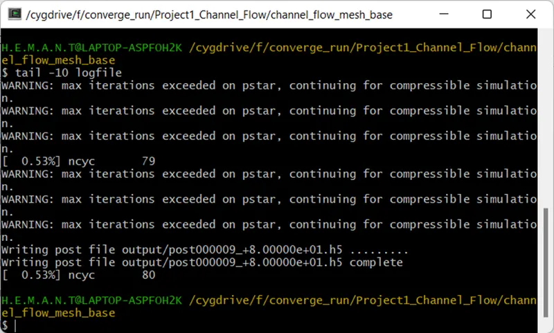
-Use the command ‘tail -10 logfile’ to get the status of the running simulation.
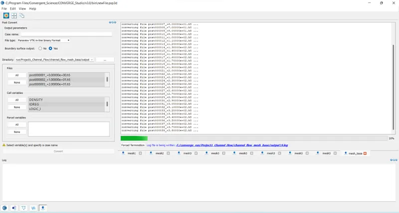
-On completion of the simulation, we need to convert the 3D output file which is readable for the Paraview.
-Open Post-Processing 3D in Converge Studio and specify the Case name. Select the Paraview VTK in-line binary Format for the File type. Select all the Post Files and Cell variables and click on Convert to complete the process.
Post-Processing:
-For post-processing, we will use the Paraview.
-Open Paraview and click on File to open the .vtm file from the Output folder. Click on OK
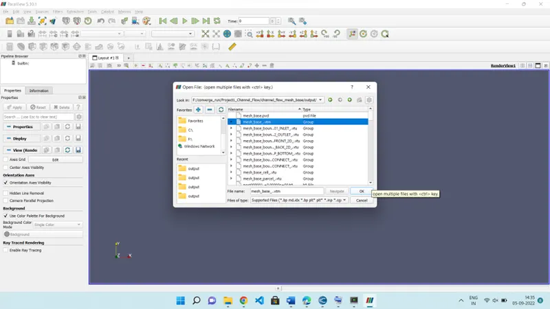
-Post-Processing is done in Paraview to obtain the plots and contours.
RESULT:
Case 1: Grid Size – 2e-4 m
Plots and Contours:
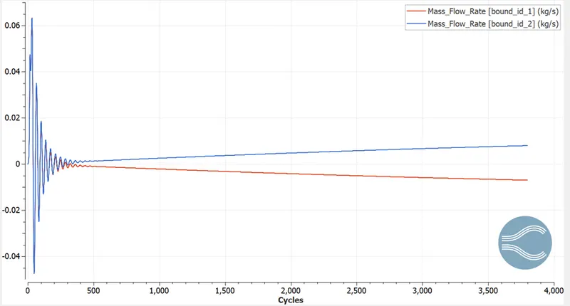
Mass Flow Rate vs Cycle (Inlet and Outlet):
Velocity:
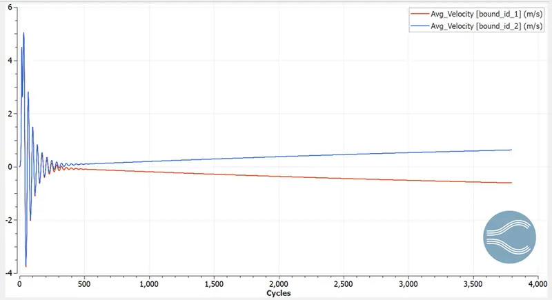
Velocity vs Cycle (Inlet and Outlet):
Velocity Contour:
Velocity Line Plot:
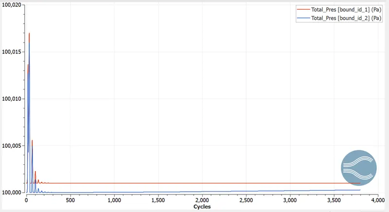
Pressure:
Pressure vs Cycle (Inlet and Outlet):
Pressure Contour:
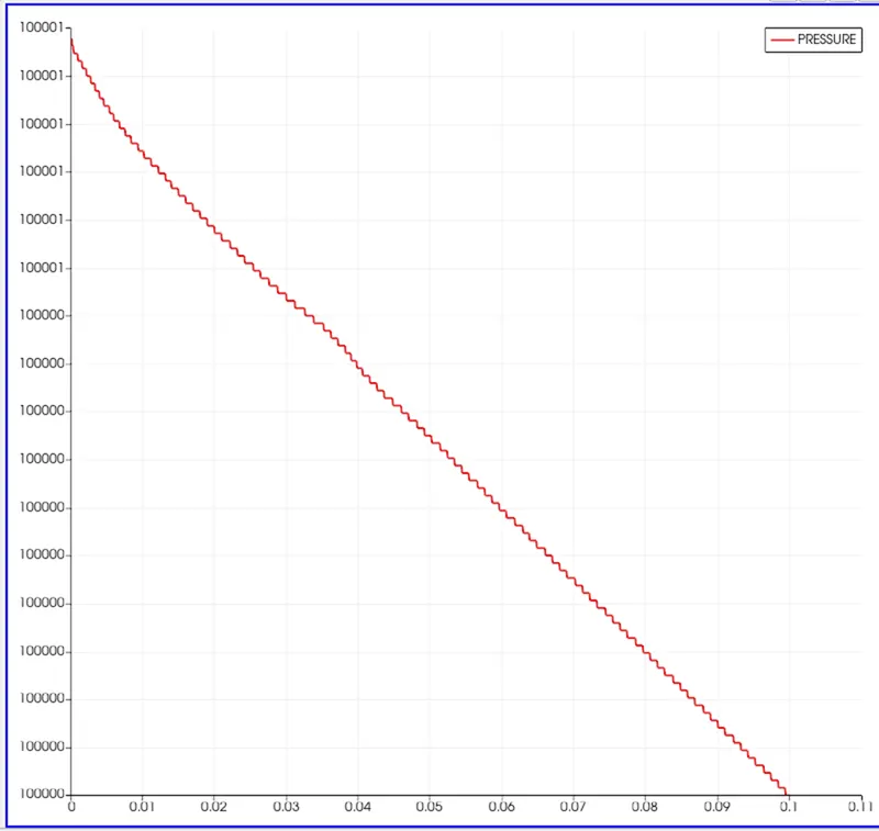
Pressure Line Plot along X-axis:
Animation:
Velocity:
Pressure:
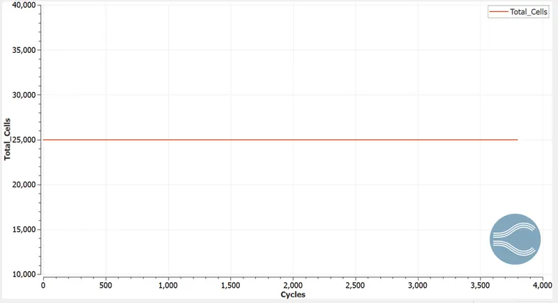
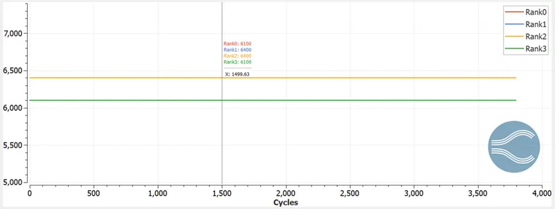
Total Cell Count:
Case 2: Grid Size – 1.5e-4 m
Plots and Contours:
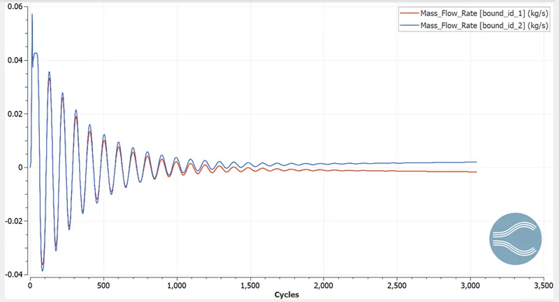
Mass Flow Rate vs Cycle (Inlet and Outlet):
Velocity:
Velocity vs Cycle (Inlet and Outlet):
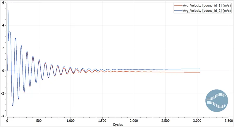
Velocity Contour:
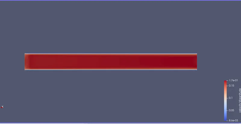
Velocity Line Plot:
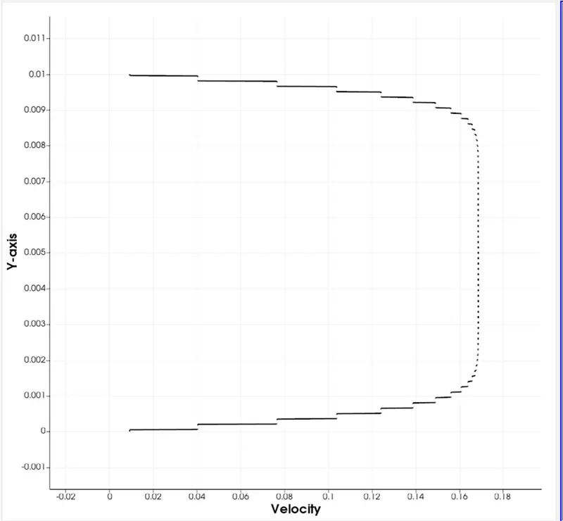
Pressure:
Pressure vs Cycle (Inlet and Outlet):
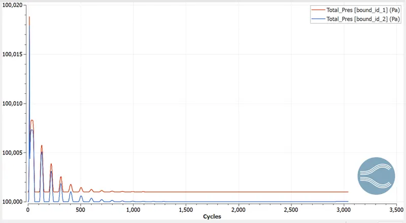
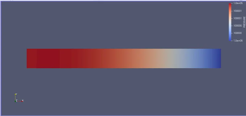
Pressure Contour:
Animation:
Velocity:
Pressure:
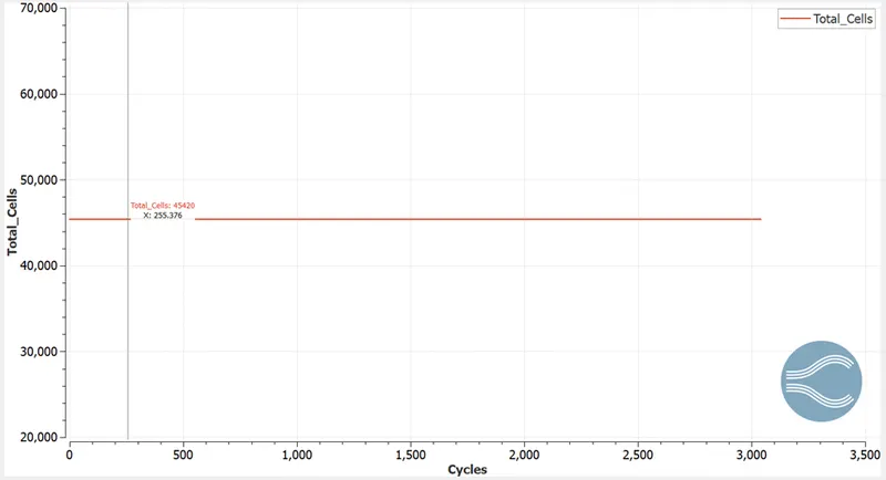
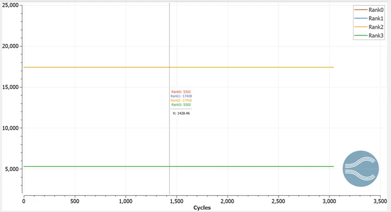
Total Cell Count:
Case 3: Grid Size – 1e-4 m
Plots and Contours:
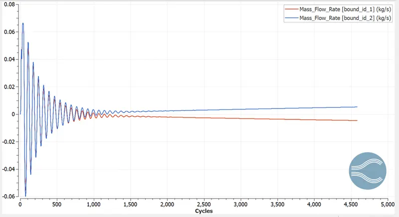
Mass Flow Rate vs Cycle (Inlet and Outlet):
Velocity:
Velocity vs Cycle (Inlet and Outlet):
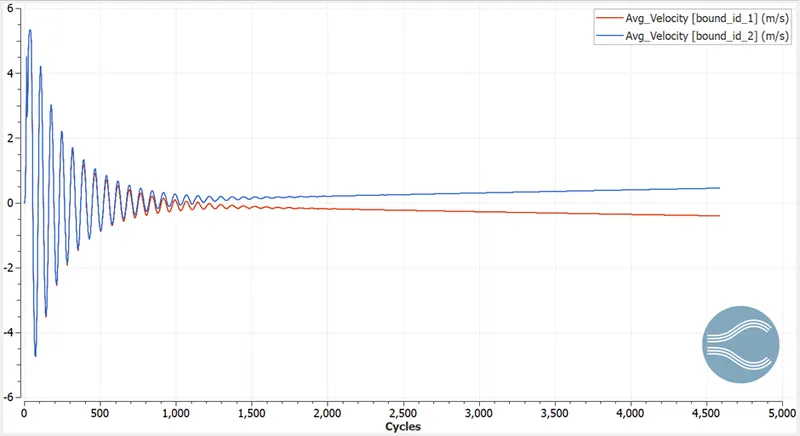
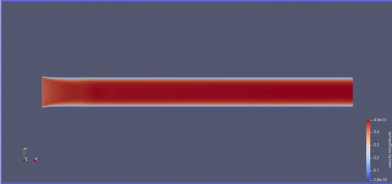
Velocity Contour:
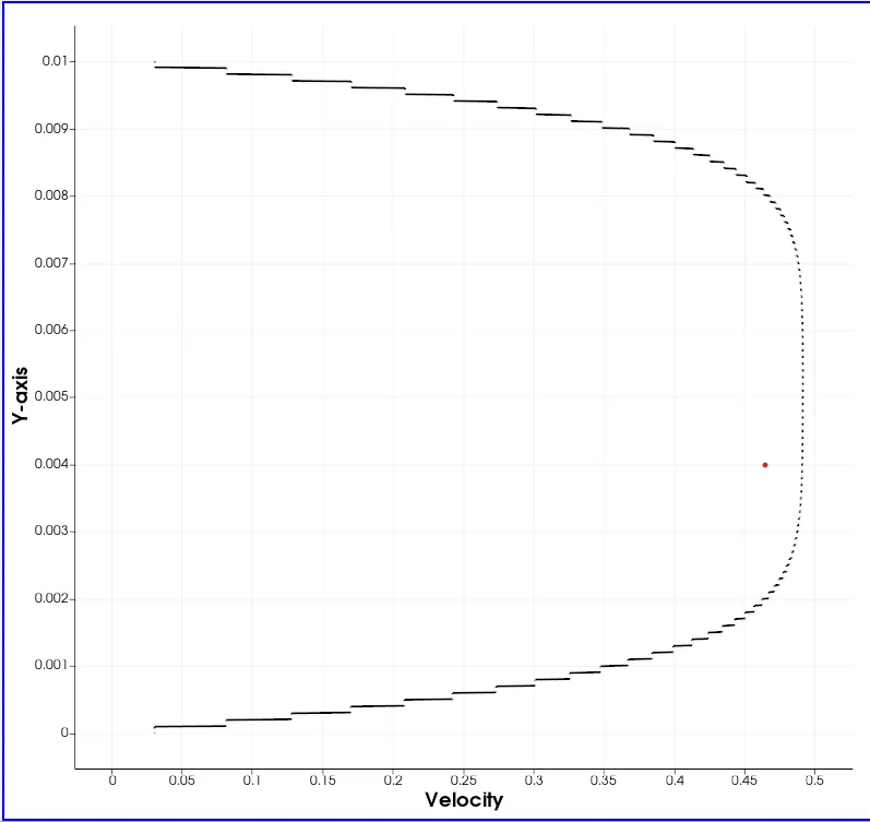
Velocity Line Plot:
Pressure:
Pressure vs Cycle (Inlet and Outlet):
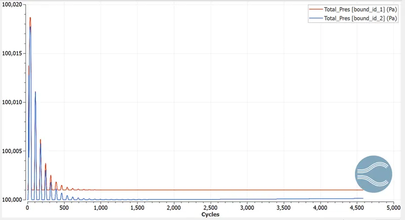
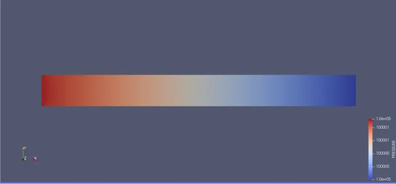
Pressure Contour:
Animation:
Velocity
Pressure:
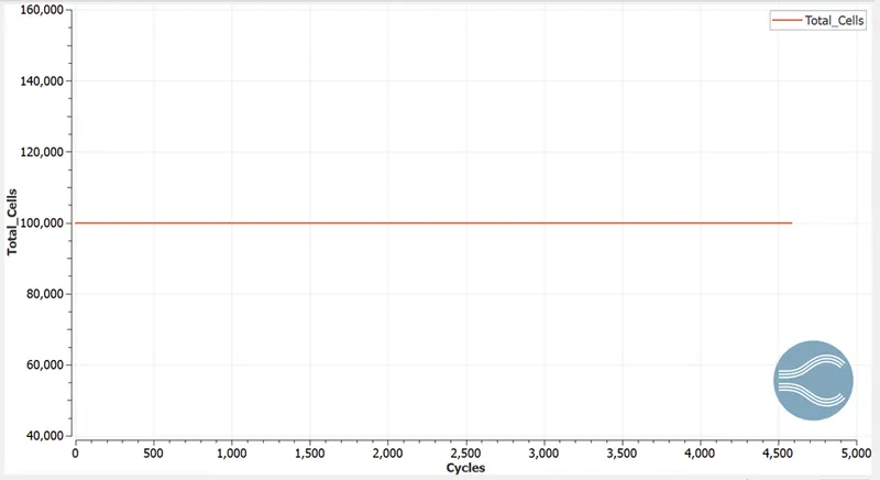
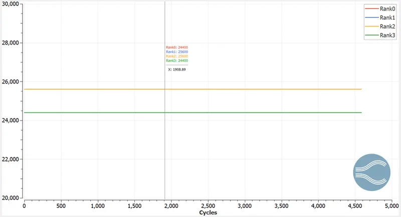
Total Cell Count:
CONCLUSION:
The channel flow simulation using Converge CFD has been performed with different mesh sizes and accurate results are obtained.