Week 5 - Genetic Algorithm

Genetic Algorithm

Aim: To find the Global Maxima for the Stalagmite function using the Genetic algorithm in MATLAB.

Objective:

• The objective of this project is to optimise and find global maxima for the stalagmite function.
• Initially, create a MATLAB script for a user-defined function which evaluates the stalagmite function.
• Use pre-defined function “ga” for genetic algorithm and evaluate global maxima for stalagmite function.
• To optimise the results, bound the search region and increase the population size.
• Create 3 cases: Unbounded Statistical Study, Statistical Study with upper and lower bound, and Bounded Statistical Study with increasing populational size.
• Compare the 3 cases with the help of outputs and plots obtained.

Introduction:

Genetic Algorithm:

A genetic Algorithm is an optimization method that is inspired by the process of natural selection. It is used to find approximate solutions to optimization and search problems. Genetic algorithms are a subset of evolutionary algorithms, which are a class of optimization and search algorithms that are based on the principles of natural evolution, such as inheritance, mutation, selection, and crossover.

The basic idea behind the genetic algorithm is to simulate the process of natural selection to find the best solution to a problem. This is done by representing potential solutions to the problem as a set of individuals, called a population. Each individual is represented by a set of genes, which are encoded as binary strings, or chromosomes. These chromosomes represent the individual's genetic makeup, and they determine fitness, or how well it solves the problem.

The genetic algorithm starts with a randomly generated initial population of individuals. It then repeatedly applies a set of genetic operators, such as crossover, mutation, and selection, to the population to generate new individuals. The unique individuals are then evaluated according to their fitness, and the best individuals are selected to form the next generation. This process is repeated until a satisfactory solution is found, or a stopping criterion is met.

The following are the general steps involved in Genetic Algorithm:

1. Define the problem: State the problem to be solved and determine the objectives and constraints.
2. Represent the solution: Choose a representation for the solutions to the problem, such as binary strings, real-valued vectors, or a combination of both.
3. Initialize the population: Generate an initial set of solutions, also known as the population. The population should be diverse and representative of the entire solution space.
4. Evaluate the fitness: Calculate the fitness of each solution in the population, using a fitness function that measures how well a solution solves the problem.
5. Select the best solutions: Choose a subset of the best solutions in the population, based on their fitness, to use in the next generation.
6. Apply genetic operators: Use genetic operators, such as crossover and mutation, to generate new solutions from the selected solutions. The genetic operators are used to maintain diversity and generate new solutions that are different from the current solutions.
7. Evaluate the new solutions: Calculate the fitness of the new solutions and add them to the population.
8. Repeat: Repeat the selection, genetic operator application, and evaluation steps for a specified number of generations or until a satisfactory solution is found.
9. Return the best solution: Return the best solution in the final population as the solution to the problem.

Methodology:

Input Function:

In this project, the Stalagmite function is used as an input function/objective function.

Mathematically, the stalagmite function is given as:

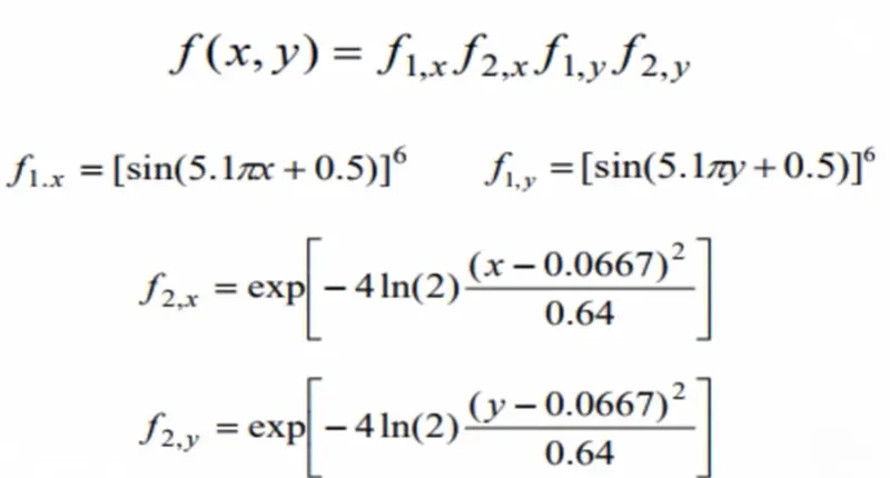
To evaluate the stalagmite function, a user-defined function is created in MATLAB. Following is the MATLAB script:

% MATLAB script for user define function to evaluate the Stalagmite function

function f = stalagmite(input_vector)

f1x = (sin(5.1*pi*input_vector(1) + 0.5)).^6;
f1y = (sin(5.1*pi*input_vector(2) + 0.5)).^6;
f2x = exp((-4*log(2)/0.64)*(input_vector(1) - 0.667).^2);
f2y = exp((-4*log(2)/0.64)*(input_vector(2) - 0.667).^2);

f = -f1x.*f2x.*f1y.*f2y;

end

Evaluation of Global Maxima:

The problem statement is to find the global maxima for the stalagmite function to obtain the same global maxima value as output for several of iterations. The search space is bounded to a definite limit in this problem.

Now, the evaluation of global maxima for the stalagmite function is done in 3 following cases:

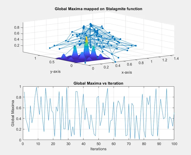
1. Case 1: Unbounded Statistical Behaviour of Genetic Algorithm: In this case, the search space is not bounded. The genetic algorithm is run for 50 iterations to observe the variation in the output.
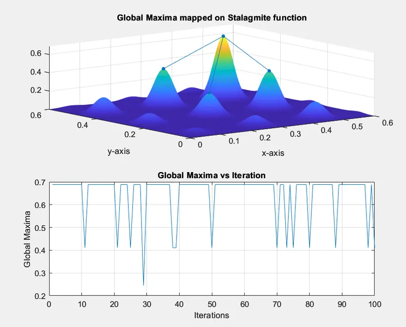
2. Case 2: Bounded Statistical Behaviour of Genetic Algorithm: The search space, for this case, is confined between the upper bound value and the lower bound value. By defining the search space, the algorithm’ search is more focused on a restricted area, which increases the probability of finding global maxima.
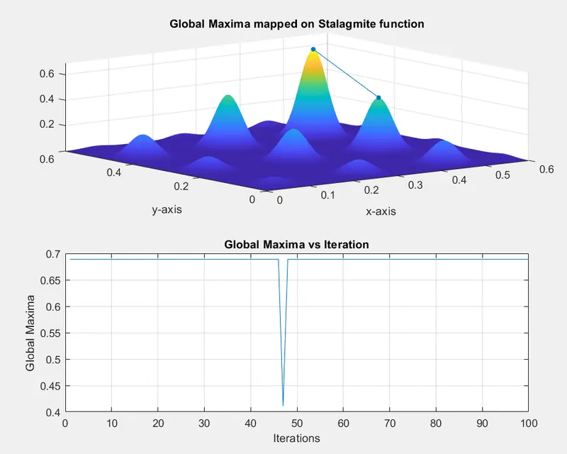
3. Case 3: Bounded Statistical Behaviour of Genetic Algorithm with increased population size: With increasing population size, a more diverse set of solutions is obtained which allows the algorithm to explore a wider range of solution space within the bounded region.

Following are the step to write a MATLAB program to find global maxima for the stalagmite function using the genetic algorithm:

1. Evaluate the global maxima of the stalagmite function using the 'ga' function for a specified number of iterations.
2. Note that the 'ga' function in MATLAB only evaluates global minima. To find the global maxima, negate the stalagmite function before evaluation, then negate the output to get the desired result.
3. Create a 3D plot and map the global maxima onto the surface plot of the stalagmite function.
4. Create a subplot to compare the global maxima with the number of iterations. This helps to visualize the accuracy and precision of the GA.
5. Repeat this process for all three cases, changing the syntax of the 'ga' function as necessary.

MATLAB Script for evaluating global maxima of the stalagmite function using the ‘ga’ function:

% MATLAB script to find the global maxima for the Stalagmite function using
% Genetic Algorithm

clear all
close all
clc

%% Creating search space and evaluating stalagmite function

% Defining the limits x-axis and y-axis
x = linspace(0,0.6,150);
y = linspace(0,0.6,150);

% Creating 2D region
[X,Y] = meshgrid(x,y);

% For loop to evaluate Stalagmite function
for i = 1: length(x)
    for j = 1: length(y)
        input_vector(1) = X(i,j);
        input_vector(2) = Y(i,j);

    Z(i,j) = -stalagmite(input_vector);
    end
end


iter = 100;  % Defining No. of Iteration to run GA

%% Case 1: Unbounded Statistical Study of Genetic algorithm

tic     % To measure the time taken by case 1

% Evaluate the global maxima of the stalagmite function using ga function 
for k = 1:iter
    [coord, fval] = ga(@stalagmite,2);    
% Above function gives two outputs: 'coord' contains the coordinates of
% function minima and 'fval' contains values of function minima
 

% Convert the function minima into global maxima by negating the output 
    x_max(k) = coord(1);
    y_max(k) = coord(2);
    z_max(k)= -fval;

end

case_1_time = toc   % 'case_1_time' variable stores the time taken for completion of case 1


% Plot for Case 1
figure (1)
subplot(2,1,1)
plot3(x_max,y_max,z_max,'Marker','.','MarkerSize',15)   % Plotting global maxima
hold on
surfc(x,y,Z)                                            % Plotting stalagmite function
shading interp
grid on
title("Global Maxima mapped on Stalagmite function")
xlabel('x-axis')
ylabel('y-axis')

% Plot for Global Maxima vs Iterations
subplot(2,1,2)

plot(z_max)
xlabel("Iterations")
ylabel("Global Maxima")
grid on
title('Global Maxima vs Iteration' )


%% Case 2: Bounded Statistical Study of Genetic Algorithm with lower and upper bounds

tic
for k = 1:iter

    [coord, fval] = ga(@stalagmite,2,[],[],[],[],[0,0],[0.6,0.6]);
% Added lower and upper bound to ga function

    x_max(k) = coord(1);
    y_max(k) = coord(2);
    z_max(k)= -fval;

end
case_2_time = toc

figure (2)
subplot(2,1,1)
plot3(x_max,y_max,z_max,'Marker','.','MarkerSize',15)   % Plotting global maxima
hold on
surfc(x,y,Z)                                            % Plotting stalagmite function
shading interp
grid on
title("Global Maxima mapped on Stalagmite function")
xlabel('x-axis')
ylabel('y-axis')

% Plot for Global Maxima vs Iterations
subplot(2,1,2)
plot(z_max)
xlabel("Iterations")
ylabel("Global Maxima")
grid on
title('Global Maxima vs Iteration' )


%% Case 3: Bounded Statistical Study of Genetic Algorithm with an increase in population size

% Created option for ga function to increase population size to 90
option = optimoptions('ga',PopulationSize=90); 

tic 
for k = 1:iter

    [coord, fval] = ga(@stalagmite,2,[],[],[],[],[0,0],[0.6,0.6],[],[],option);
    x_max(k) = coord(1);
    y_max(k) = coord(2);
    z_max(k)= -fval;

end
case_3_time = toc

figure (3)
subplot(2,1,1)
plot3(x_max,y_max,z_max,'Marker','.','MarkerSize',15)   % Plotting global maxima
hold on
surfc(x,y,Z)                                            % Plotting stalagmite function
shading interp
grid on
title("Global Maxima mapped on Stalagmite function")
xlabel('x-axis')
ylabel('y-axis')

% Plot for Global Maxima vs Iterations
subplot(2,1,2)

plot(z_max)
xlabel("Iterations")
ylabel("Global Maxima")
grid on
title('Global Maxima vs Iteration' )


%% Result

fprintf('\n Case 1: Unbounded Statistical Study of Genetic algorithm')
fprintf('\n The time taken for the Case 1 is : %f',case_1_time)

fprintf('\n Case 2: Bounded Statistical Study of Genetic Algorithm with lower and upper bounds')
fprintf('\n The time taken for the Case 2 is : %f',case_2_time)

fprintf('\n Case 3: Bounded Statistical Study of Genetic Algorithm with increase in population size')
fprintf('\n The time taken for the Case 3 is : %f',case_3_time)

‘ga’ function:

The general syntax for the ‘ga’ function in MATLAB is

[x, fval] = ga(fun,nvar,A,b,Aeq,beq,lb,ub,nonlcon,option)

Input arguments:

‘fun’ is the objective function to be minimized. The objective function should take a single input argument and return a value that represents the solution.

‘nvar’ is the number of variables.

‘A’ and ‘b’ are input arguments representing linear inequality constraints in the form of ‘A*x <= b’

‘Aeq’ and ‘beq’ are input arguments representing linear equality constraints in the form of ‘A*x < = b’ and ‘Aeq*x = beq’. Both the input arguments are used when there is any linear inequality constraint.

‘lb’ and ‘ub’ are the lower and upper bound such that lb<= x<=ub.

‘nonlcon’ represents the non-linear constraint

‘option’ represents the options in the ga function created using ‘optimoption’. ‘option’ contains information for additional modification in the ‘ga’ function.

Output argument:

‘x’ represents of the optimal solution of the ‘ga’ function. In the project, ‘x’ is the coordinates of local minima.

‘fval’ represents the value of the objective function at ‘x’. In the project, ‘fval’ is the functional value of local minima.

Results:

Case 1:

Case 2:

Case 3:

Conclusion:

Bounding the search space for the genetic algorithm helps in reducing the noise in the output. increasing the population size leads to an increase in the probability of finding the optimum solution.