Week 5.1 - Mid term project - Solving the steady and unsteady 2D heat conduction problem
Solving study and transient state 2D heat conduction using MATLAB
The heat equation is a partial differential equation that describes the heat distribution in the material with respect to time and space
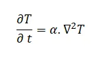
where `alpha` is the thermal diffusivity of the material or the medium.
Steady-state
A system is said to be in a steady state if the state of the system does not change with respect to time.
So the steady-state equation is
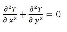
as
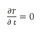
the steady-state heat transfer equation is an elliptical PDE. This equation is discretized using the Central difference scheme
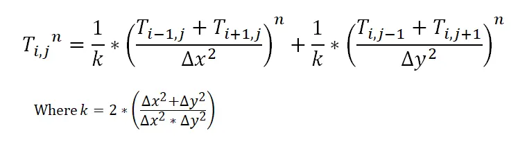
the discretized steady-state equation is

Where and i, j represent the position, and n represent the nth number of the time steps. Note that 'n' is a superscript not exponential.
On simplifying the above equation,
Unsteady State
The transient/unsteady-state heat transfer equation for a 2D isotropic and homogeneous material is
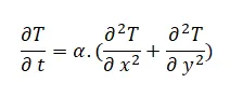
Though the transient state heat equation is a parabolic PDE when the time reaches to infinity, the time derivative tends to zero and the material attains a steady state.
So it is concluded that the above equation is parabolic in time and elliptical in space.
Since Parabolic PDEs represent time marching problems and are discretized using the Forward difference scheme.
Whereas Elliptical PDEs represents Steady-state problems and are discretized using the Central difference scheme
The discretized unsteady-state equation is

Where i, j represent the position and n represent the nth number of the time steps. Note that 'n' is a superscript not exponential.
This equation can be further written in implicit and explicit forms. Solving the convective term for the nth time step gives explicit form and for the n+1th time step gives the implicit form of the equation.
On simplifying Explicit Form,

Explicit equations are easy to solve. Solution for Explicit equations is obtained with the direct method.
and On simplifying Implicit form,
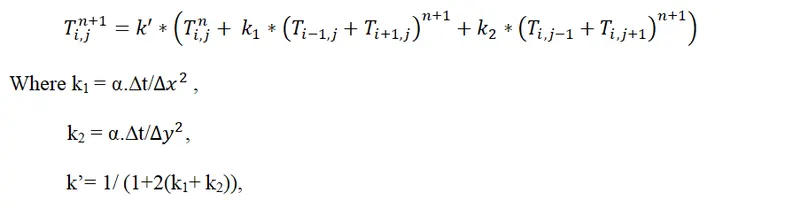
For Implicit equations, the solution is obtained using iterative methods. Jacobi Method, Gauss-Seidel Method, and Successive Over Relaxation Method are some of the examples of iteration method, which are used in this project to solve the implicit equation.
MATLAB Programs
I wrote individual and independent MATLAB script for all the method. Primarily all scripts have a common structure wherein the first section I defined dimensions of the mesh/domain. In the second section, I defined boundary temperature conditions. Given data
Top Boundary = 600 K
Bottom Boundary = 900 K
Left Boundary = 400 K
Right Boundary = 800 K
I assume 700K as the initial guess temperature.
And Error tolerance = 1e-4.
Third section deals with the calculation. This section differs for different methods. The last section is plotting.
In Jacobi Method, we will calculate the current temperature using the Temperature values of the previous iteration.
In Gauss-Seidel Method, we will calculate the current temperature using the updated Temperature values obtained from the previous iteration.
In the Successive Over Relaxation Method, the current temperature value is calculated using the sum of temperature values of the previous iteration and product of the rate of change of temperature and an over-relaxation factor.
Steady-State
1) Jacobi Method
% Solving 2-D Steady State Heat Conduction Problem Using Jacobi Method
close all
clear all
clc
% Defining the Domain
 % No. of Grid points
nx=20;
ny=nx;

% Total Domain Length
x=linspace(0,1,nx);
y=x;

% Grid Size
dx=x(2)-x(1);
dy=y(2)-y(1);

% Creating Meshgrid in Domain
[X,Y]=meshgrid(x,y);

% Defining Conditions
% Creating a Matrix which represents the Temperature distribution

T=700*ones(nx,ny);                   % Assuming initial temperature as 700K
T(:,1)=400;                          % Left Boundary Condition
T(:,nx)=800;                         % Right Boundary Condition
T(1,:)=600;                          % Top Boundary Condition
T(ny,:)=900;                         % Bottom Boundary Condition
T(1,1)= (T(1,2)+T(2,1))/2;           % Top Left Corner Boundary Condition
T(1,nx)=(T(1,nx-1)+T(2,nx))/2;       % Top Right Boundary Condition
T(ny,1)=(T(ny-1,1)+T(ny,2))/2;       % Bottom Left Corner Boundary Condition
T(nx,ny)=(T(ny,nx-1)+T(ny-1,nx))/2;  % Bottom Right Corner Boundary Condition

T_old=T;

% Error and Tolerance
error=1;
tol=1e-4;
iteration_count=1;
% Calculation

% Jacobi Method

while (error>tol)  % Convergence Loop

for i=2:nx-1       % Space Loop
    for j=2:ny-1
  k= 2*((dx^2+dy^2)/(dx*dy)^2);

  T(i,j)= (T_old(i-1,j)+T_old(i+1,j))/(k*dx^2) + (T_old(i,j-1)+T_old(i,j+1))/(k*dy^2);
    end
end
error=max(max(abs(T-T_old)));
T_old=T;                      % Updating temperatures
iteration_count=iteration_count+1;
% plot


contourf(X,Y,T,'Linestyle','none')
        title(['Jacobi Method (Implict)'],['Iterations = ',num2str(iteration_count)])
colorbar
set(gca,'ydir','reverse')
pause(1/240)
end
2) Gauss-Seidel Method
% Solving 2-D Steady State Heat Conduction Problem Using Gauss-Seidel Method
close all
clear all
clc
% Defining the Domain
 % No. of Grid points
nx=20;
ny=nx;

% Total Domain Length
x=linspace(0,1,nx);
y=x;

% Grid Size
dx=x(2)-x(1);
dy=y(2)-y(1);

% Creating Meshgrid in Domain
[X,Y]=meshgrid(x,y);

% Defining Conditions
% Creating a Matrix which represents the Temperature distribution

T=700*ones(nx,ny);                   % Assuming initial temperature as 700K
T(:,1)=400;                          % Left Boundary Condition
T(:,nx)=800;                         % Right Boundary Condition
T(1,:)=600;                          % Top Boundary Condition
T(ny,:)=900;                         % Bottom Boundary Condition
T(1,1)= (T(1,2)+T(2,1))/2;           % Top Left Corner Boundary Condition
T(1,nx)=(T(1,nx-1)+T(2,nx))/2;       % Top Right Boundary Condition
T(ny,1)=(T(ny-1,1)+T(ny,2))/2;       % Bottom Left Corner Boundary Condition
T(nx,ny)=(T(ny,nx-1)+T(ny-1,nx))/2;  % Bottom Right Corner Boundary Condition

T_old=T;

% Error and Tolerance
error=1;
tol=1e-4;
iteration_count=1;
% Calculation
  % Gauss-Seidel Method
while (error>tol) % Convergence Loop

for i=2:nx-1       % Space Loop
    for j=2:ny-1
  k= 2*((dx^2+dy^2)/(dx*dy)^2);

    T(i,j)= (T(i-1,j)+T(i+1,j))/(k*dx^2) + (T(i,j-1)+T(i,j+1))/(k*dy^2);
    end
end
error=max(max(abs(T-T_old)));
T_old=T;                      % Updating temperatures
iteration_count=iteration_count+1;
% plot


contourf(X,Y,T,'Linestyle','none')
        title(['Gauss-Seidel Method (Implict)'],['Iterations = ',num2str(iteration_count)])
colorbar
set(gca,'ydir','reverse')
pause(1/240)
end
3) SOR Method
% Solving 2-D Steady State Heat Conduction Problem Using SOR Method

close all
clear all
clc
%Defining Domain Size
 % No. of Grid points
nx=20;
ny=nx;

% Total Domain Length
x=linspace(0,1,nx);
y=x;

% Grid Size
dx=x(2)-x(1);
dy=y(2)-y(1);

% Creating Meshgrid in Domain
[X,Y]=meshgrid(x,y);

% Defining Conditions
% Creating a Matrix which represents the Temperature distribution

T=700*ones(nx,ny);                   %Assuming initial tempaerature as 700K
T(:,1)=400;                          % Left Boundary Condition
T(:,nx)=800;                         % Right Boundary Condition
T(1,:)=600;                          % Top Boundary Condition
T(ny,:)=900;                         % Bottom Boundary Condition
T(1,1)= (T(1,2)+T(2,1))/2;           % Top Left Corner Boundary Condition
T(1,nx)=(T(1,nx-1)+T(2,nx))/2;       % Top Right Boundary Condition
T(ny,1)=(T(ny-1,1)+T(ny,2))/2;       % Bottom Left Corner Boundary Condition
T(nx,ny)=(T(ny,nx-1)+T(ny-1,nx))/2;  % Bottom Right Corner Boundary Condition

T_old=T;

% Error and Tolerance
error=1;
tol=1e-4;

iteration_count=1;

% Relaxation Factor
w=1.714;

% Succesive Over Relaxation Method

while (error>tol) % Convergence Loop

  for i=2:nx-1    % Space Loop
    for j=2:ny-1

  k= 2*((dx^2+dy^2)/(dx*dy)^2);

    T(i,j)= (T(i-1,j)+T(i+1,j))/(k*dx^2) + (T(i,j-1)+T(i,j+1))/(k*dy^2);

  T(i,j)= (1-w)*T_old(i,j) + w*T(i,j);
    end
  end
error=max(max(abs(T-T_old)));
T_old=T;
iteration_count=iteration_count+1;

% plot
contourf(X,Y,T,'Linestyle','none')
title(['SOR Method (Implict)'],['Iterations = ',num2str(iteration_count)])
colorbar
set(gca,'ydir','reverse')
pause(1/240)
end
Plots and Results
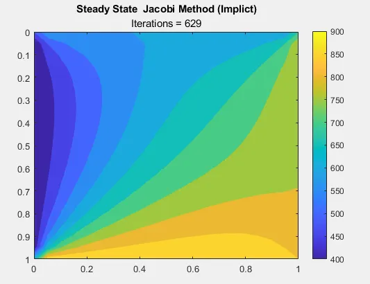
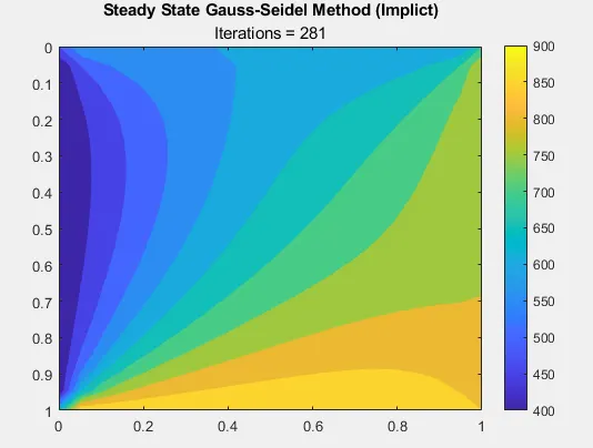
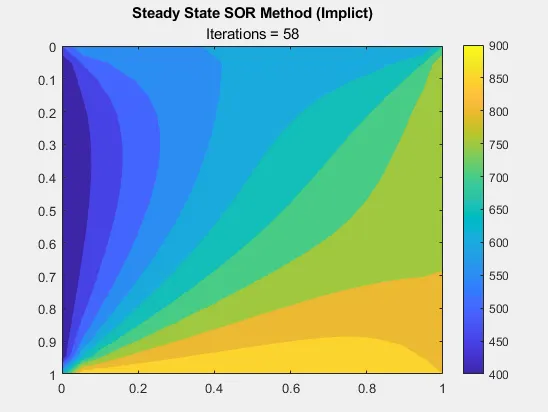
For the SOR method over-relaxation factor is 1.714.
Unsteady-State
Codes have a similar structure to the previous one but here there is the inclusion of the time loop in the codes.
In order to satisfy the CFL criterion, the value of thermal diffusivity for the Explicit method is 0.0068.
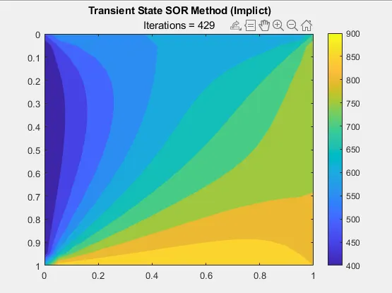
For the remaining methods, thermal diffusivity is 1.4 and simulation time is 20 sec with 2000 timesteps.
Explicit
% Solving 2-D Transient Heat Conduction Problem Using Explict Method
close all
clear all
clc
%Defining Domain Size
 % No. of Grid points
nx=20;
ny=nx;

% Domain Length
x=linspace(0,1,nx);
y=x;

% Each Grid Size
dx=x(2)-x(1);
dy=y(2)-y(1);

% Creating Meshgrid in Domain
[X,Y]=meshgrid(x,y);

% Define Time
dt=1e-1;
t=20;
nt=t/dt;

% Creating Meshgrid in Domain
[X,Y]=meshgrid(x,y);

% Defining Conditions
% Creating a Matrix which represents the Temperature distribution

T=700*ones(nx,ny);                   % Assuming initial temperature as 700K
T(:,1)=400;                          % Left Boundary Condition
T(:,nx)=800;                         % Right Boundary Condition
T(1,:)=600;                          % Top Boundary Condition
T(ny,:)=900;                         % Bottom Boundary Condition
T(1,1)= (T(1,2)+T(2,1))/2;           % Top Left Corner Boundary Condition
T(1,nx)=(T(1,nx-1)+T(2,nx))/2;       % Top Right Boundary Condition
T(ny,1)=(T(ny-1,1)+T(ny,2))/2;       % Bottom Left Corner Boundary Condition
T(nx,ny)=(T(ny,nx-1)+T(ny-1,nx))/2;  % Bottom Right Corner Boundary Condition


T_old=T;

% CFL numbers
alpha=0.006;  % Thermal diffusivity
kx=alpha*(dt/dx^2);
ky=alpha*(dt/dy^2);

% Time Loop
 for s=1:nt
  % Space Loop
   for i=2:nx-1
    for j=2:ny-1

     H= T(i-1,j)+T(i+1,j); % Horizontal Grids
     V= T(i,j-1)+T(i,j+1); % Vertical   Grids

  T(i,j)=(1-2*kx-2*ky)*T_old(i,j)+ kx*(H) + ky*(V);
    end
   end

% Plot
contourf(X,Y,T,'Linestyle','none')
title(['Transient State (Explict)'],['Time = ',num2str(s*dt),' s'])
colorbar
set(gca,'ydir','reverse')
pause(1/240)

T_old=T;
 end
Implicit Methods
1) Jacobi Method
% Solving 2-D Transient Heat Conduction Problem Using Jacobi Method
close all
clear all
clc
%Defining Domain Size
 % No. of Grid points
nx=20;
ny=nx;

% Total Domain Length
x=linspace(0,1,nx);
y=linspace(0,1,ny);

% Grid Size
dx=x(2)-x(1);
dy=y(2)-y(1);

% Creating Meshgrid in Domain
[X,Y]=meshgrid(x,y);
% Time step
dt=1e-1;
t=20;
nt=t/dt;

% Defining Conditions
% Creating a Matrix which represents the Temperature distribution

T=700*ones(nx,ny);                   %Assuming initial tempaerature as 700K
T(:,1)=400;                          % Left Boundary Condition
T(:,nx)=800;                         % Right Boundary Condition
T(1,:)=600;                          % Top Boundary Condition
T(ny,:)=900;                         % Bottom Boundary Condition
T(1,1)= (T(1,2)+T(2,1))/2;           % Top Left Corner Boundary Condition
T(1,nx)=(T(1,nx-1)+T(2,nx))/2;       % Top Right Boundary Condition
T(ny,1)=(T(ny-1,1)+T(ny,2))/2;       % Bottom Left Corner Boundary Condition
T(nx,ny)=(T(ny,nx-1)+T(ny-1,nx))/2;  % Bottom Right Corner Boundary Condition

T_old=T;
T_prev=T;
T_intial=T;

% Error and Tolerance
error=1;
tol=1e-4;

% CFL numbers
alpha=0.14;
kx=alpha*(dt/dx^2);
ky=alpha*(dt/dy^2);
k= 1/(1+2*(kx+ky));
iter_count=1;

%Time loop
for s=1:nt
while error>tol
   for i=2:nx-1
    for j=2:ny-1

           H= (T_old(i-1,j)+T_old(i+1,j)); % Horizontal Grids
           V= (T_old(i,j-1)+T_old(i,j+1)); % Vertical   Grids

            T(i,j)= k*(T_prev(i,j)+ kx*(H) +ky*(V));
    end
   end
   error=max(max(abs(T_old-T)));  % Calculating error
T_old=T;                          % Updating old Temperature values
iter_count=iter_count+1;
end
contourf(X,Y,T,'Linestyle','none')
title(['Transient State Jacobi (Implict)'],['Iteration = ',num2str(iter_count)])
colorbar
set(gca,'ydir','reverse')
pause(1/240)

error=1;       % Updating error value
T_prev=T;      % Updating old Temperature values for next time step
end
2) Gauss-Seidel Method
% Solving  Transient state heat equation using Gauss-Seidel Method
close all
clear all
clc
%Defining Domain Size
 % No. of Grid points
nx=20;
ny=nx;

% Total Domain Length
x=linspace(0,1,nx);
y=x;

% Grid Size
dx=x(2)-x(1);
dy=y(2)-y(1);

% Creating Meshgrid in Domain
[X,Y]=meshgrid(x,y);
% Time step
dt=1e-1;
t=20;
nt=t/dt;

% Defining Conditions
% Creating a Matrix which represents the Temperature distribution

T=700*ones(nx,ny);                   %Assuming initial temperature as 700K
T(:,1)=400;                          % Left Boundary Condition
T(:,nx)=800;                         % Right Boundary Condition
T(1,:)=600;                          % Top Boundary Condition
T(ny,:)=900;                         % Bottom Boundary Condition
T(1,1)= (T(1,2)+T(2,1))/2;           % Top Left Corner Boundary Condition
T(1,nx)=(T(1,nx-1)+T(2,nx))/2;       % Top Right Boundary Condition
T(ny,1)=(T(ny-1,1)+T(ny,2))/2;       % Bottom Left Corner Boundary Condition
T(nx,ny)=(T(ny,nx-1)+T(ny-1,nx))/2;  % Bottom Right Corner Boundary Condition

T_old=T;
T_prev=T;

% Error and Tolerance
error=1;
tol=1e-4;
k1=(dt/dx^2);
k2=(dt/dy^2);
k3= 1/(1+2*(k1+k2));
 iter_count=1;

%   Time loop
for s=1:nt
    while (error>tol) % Convergence Loop
   for i=2:nx-1        % Space Loop
    for j=2:ny-1
     T_L= T(i-1,j);
     T_R= T(i+1,j);
     T_T= T(i,j-1);
     T_B= T(i,j+1);

  T(i,j)= k3*(T_prev(i,j)+ k1*(T_L+T_R) + k2*( T_T+T_B));
    end
     end
error=max(max(abs(T-T_old)));  % Calulating error value
T_old=T;                       % Updating old Temperature values
iter_count=iter_count+1;
 end

contourf(X,Y,T,'Linestyle','none')
title(['Transient State Gauss-Seidel Method (Implict)'],['Iterations =',num2str(iter_count)])
colorbar
set(gca,'ydir','reverse')
pause(1/240)
error=1;       % Updating error value
T_prev=T;      % Updating old Temperature values for next time step
end
3) SOR Method
% Solving  2-D Transient state Heat Conduction Problem using SOR Method
close all
clear all
clc
%Defining Domain Size
 % No. of Grid points
nx=20;
ny=nx;

% Total Domain Length
x=linspace(0,1,nx);
y=x;

% Grid Size
dx=x(2)-x(1);
dy=y(2)-y(1);

% Creating Meshgrid in Domain
[X,Y]=meshgrid(x,y);
% Time step
dt=1e-1;
t=20;
nt=t/dt;

% Defining Conditions
% Creating a Matrix which represents the Temperature distribution

T=700*ones(nx,ny);                   %Assuming initial tempaerature as 700K
T(:,1)=400;                          % Left Boundary Condition
T(:,nx)=800;                         % Right Boundary Condition
T(1,:)=600;                          % Top Boundary Condition
T(ny,:)=900;                         % Bottom Boundary Condition
T(1,1)= (T(1,2)+T(2,1))/2;           % Top Left Corner Boundary Condition
T(1,nx)=(T(1,nx-1)+T(2,nx))/2;       % Top Right Boundary Condition
T(ny,1)=(T(ny-1,1)+T(ny,2))/2;       % Bottom Left Corner Boundary Condition
T(nx,ny)=(T(ny,nx-1)+T(ny-1,nx))/2;  % Bottom Right Corner Boundary Condition

T_old=T;
T_prev=T;

% Error and Tolerance
error=1;
tol=1e-4;
k1=(dt/dx^2);
k2=(dt/dy^2);
k3= 1/(1+2*(k1+k2));

% Relaxation Factor
w=1.7;

 iter_count=1;

%   Time loop
for s=1:nt
   while (error>tol)
   for i=2:nx-1
    for j=2:ny-1
     T_L= T(i-1,j);
     T_R= T(i+1,j);
     T_T= T(i,j-1);
     T_B= T(i,j+1);

  T(i,j)= k3*(T_prev(i,j)+ k1*(T_L+T_R) + k2*( T_T+T_B));
    T(i,j)= (1-w)*T_old(i,j) + w*T(i,j);
    end
   end

   error=max(max(abs(T_old-T)));  % Calculating error
T_old=T;                          % Updating old Temperature values
iter_count=iter_count+1;
   end
% Plot
contourf(X,Y,T,'Linestyle','none')
title(['Transient State SOR Method (Implict)'],['Iterations = ',num2str(iter_count)])
colorbar
set(gca,'ydir','reverse')
pause(1/240)

error=1;       % Updating error value
T_prev=T;      % Updating old Temperature values for next time step
end
Plots
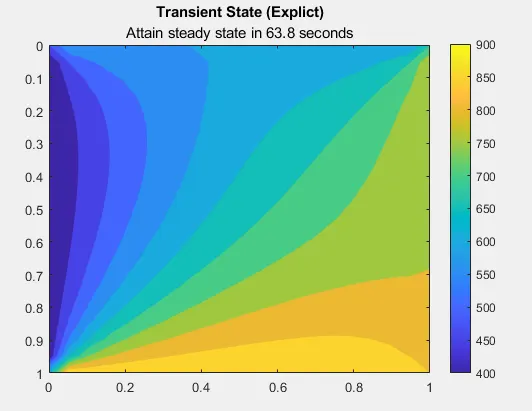
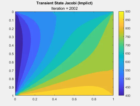
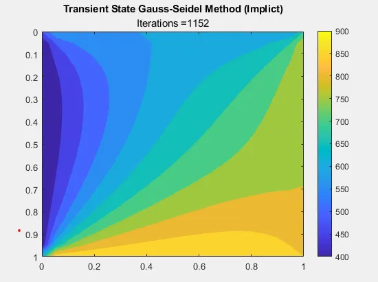
Conclusion
It is observed that solution for transient state using explicit method became unstable when CFL value exceeds the threshold limit i.e. `alpha(dt/(Deltax^2) + dt/(Delta y^2)) <= 0.5`. For implicit methods, the CFL value does not affect the stability of the solution.