Week 4.2: Project - Transient simulation of flow over a throttle body

Transient state simulation of flow over a throttle body

Aim:

To set up and run the transient state simulation for flow over the throttle body using Converge.

Objective:

• The objective of this project is to set up the transient-state simulation for flow over throttle using Converge Studio and run the simulation using Converge.
• The STL model of the Elbow pipe with a Butterfly valve is used for the simulation.
• The purpose of this simulation is to observe the effect of the throttle on the flow through the elbow pipe. The butterfly valve will act as the throttle for this simulation.
• In this simulation, the throttle valve will start from a fully open profile, rotates (close) up to 25 degrees, and come back to its original position.
• Post-process the result using Paraview

Introduction:

Introduction:

A throttle is a mechanism used to control the fluid flow through a pipe by constricting or obstructing the flow.

A throttle mechanism is placed in the air-fuel intake manifold of the internal combustion engine to control the amount of air-fuel mixture flowing into the combustion chamber.

Mostly in the internal combustion engine, the Butterfly valve is used as a throttle body. A butterfly valve is a quarter-turn rotational valve which has a disc mounted on a rotational shaft.

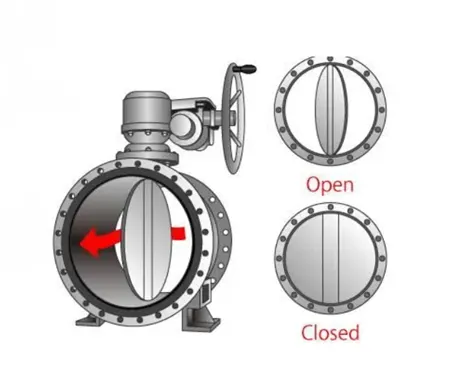
Its simple mechanism, very easy to operate and quick response make it ideal for the throttle for an IC engine.

In the following simulation, we will analyse the effect of the throttle body on the fluid flow when it rotates to restrict the fluid flow.

Procedure:

Simulation setup in the Converge Studio:

• Import the CAD model (STL file) of the elbow pipe into the Converge Studio.
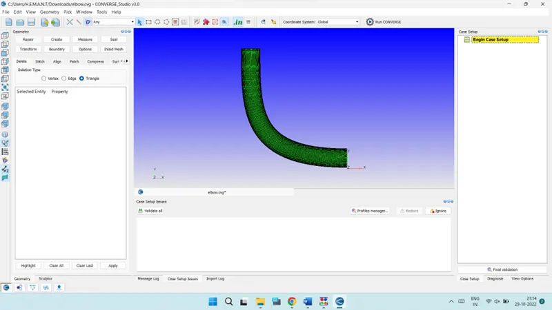
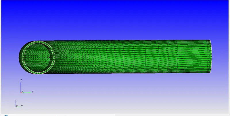
• Delete the outer wall of the pipe as they have no purpose in the current simulation.

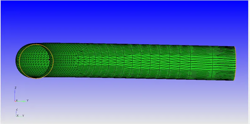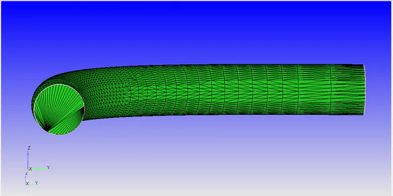
• Close the open edges to create a water-tight geometry.
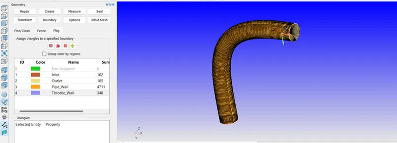
• Define the boundaries and assign the name for the boundaries.
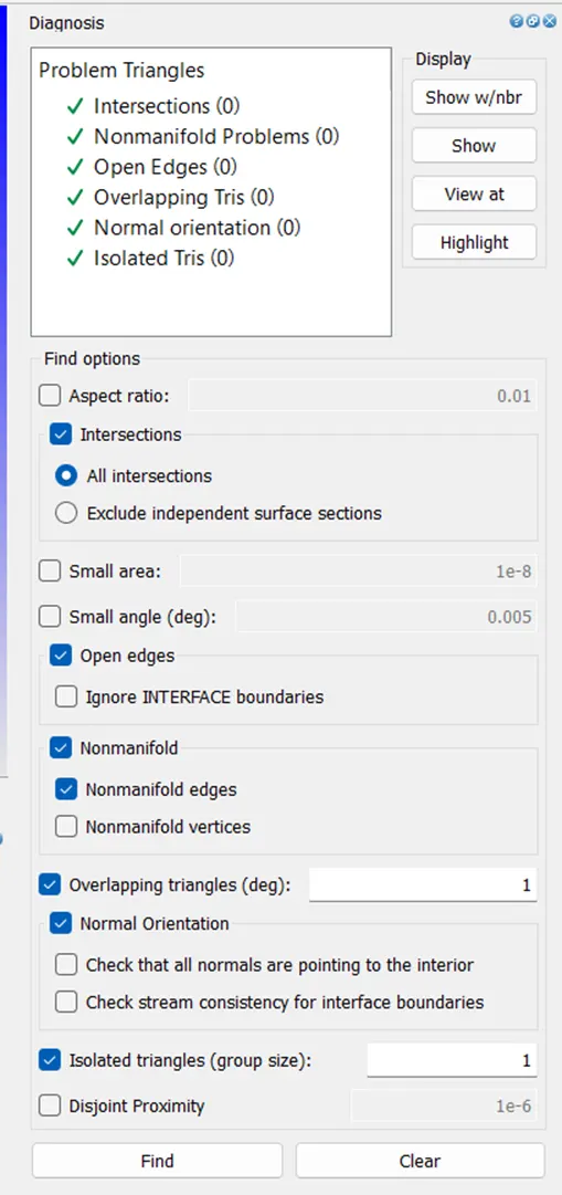
• Perform a diagnostic test to look for geometrical errors if any.
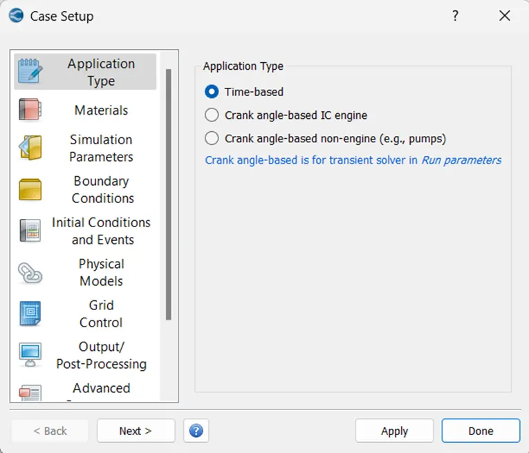
• Begin the case setup for the simulation with the Application type as Time-based.
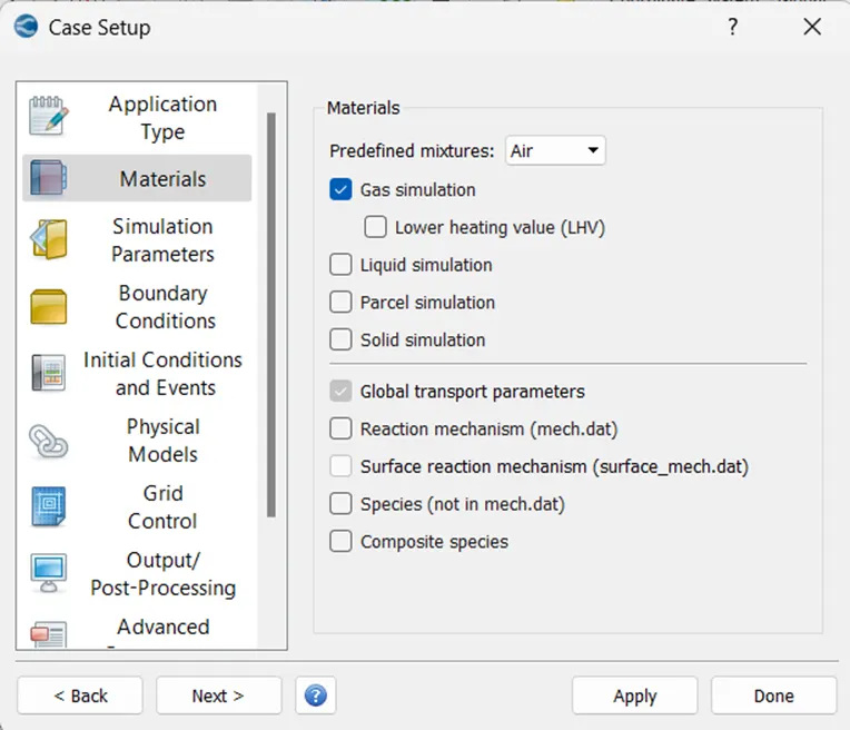
• For the Materials, set Air as a Pre-defined mixture and uncheck all the options except Gas simulation as we are interested in gas simulation only.
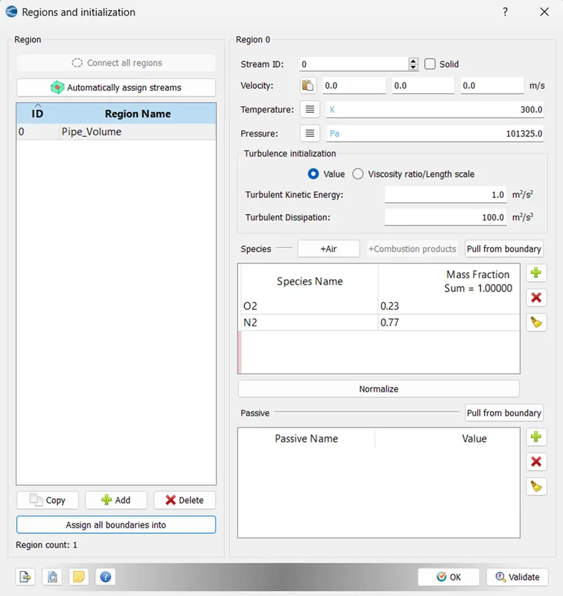
• For the initial condition, assign the region inside the pipe.
• Set up the boundary condition for each boundary.

BOUNDARY CONDITION

Inlet

1. Boundary Type: INFLOW
2. Pressure: 1.5 Mpa
3. Velocity: Zero Normal Gradient
4. Temperature: 300 K
5. Species: Air

Outlet

1. Boundary Type: OUTFLOW
2. Pressure: 1 Mpa
3. Velocity: Zero Normal Gradient
4. Temperature: 300 K
5. Species: Air

Pipe Wall

1. Boundary Type: WALL
2. Wall motion type: Stationary
3. Surface movement: Fixed
4. Law of Wall
5. Temperature: Zero Normal Gradient
6. Turbulent Kinetic Energy:
7. Turbulent Dissipation: Wall Model
8. Near Wall Treatment: Global

• To set up a rotating motion boundary condition for the throttle wall, coordinates of the rotation center and rotation axis are required.
• In the Measure tool, by using the Location option, find the co-ordinate of the cell in the center of the throttle body, which will act as a rotation center.
• Similarly, for the rotation axis, use the Direction option, to find the cell normal.

• Boundary Condition for Throttle Wall

Throttle Wall

1. Boundary Type: WALL
2. Wall motion type: Rotating
3. Surface movement: MOVING
4. Law of Wall
5. Temperature: Zero Normal Gradient
6. Turbulent Kinetic Energy:
7. Turbulent Dissipation: Wall Model
8. Near Wall Treatment: Global
9. Paste the coordinates for the rotation center and axis, found using the Measure tool.

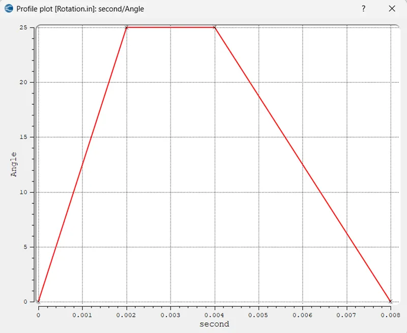
• For the rotation rate of the throttle, check (tick) the Use File option and create a Rotation.in input file as explained in the table below.

Time (milliseconds)	Angle of rotation
0	0
2	25
4	25
8	0

• Profile plot for the angle of rotation vs second is given below.
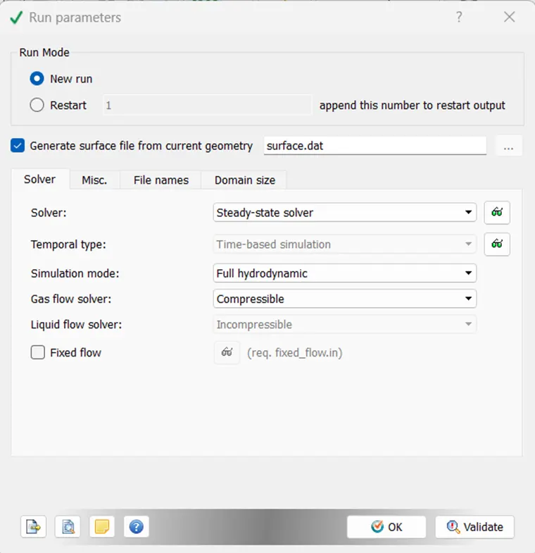
• In the Run Parameters, choose Transient solver for the solver and Full hydrodynamic for simulation mode as shown in the figure below.

• Determine the end time for the simulation before setting up the Simulation Parameter.

• To calculate the end time, determine the fluid velocity and distance travelled by the fluid in the elbow pipe.

• On observing the dimensions of the elbow pipe, the fluid travels approximately 0.125m in the pipe and the average fluid velocity at the outlet obtained from steady-state simulation is 225 m/s approx.

• Time taken for fluid to travel from inlet to outlet is time = distance/velocity. 125/225 = 5.5e-4 s

• Want to simulate the flow 20 times then the end time will be 0.01 s.

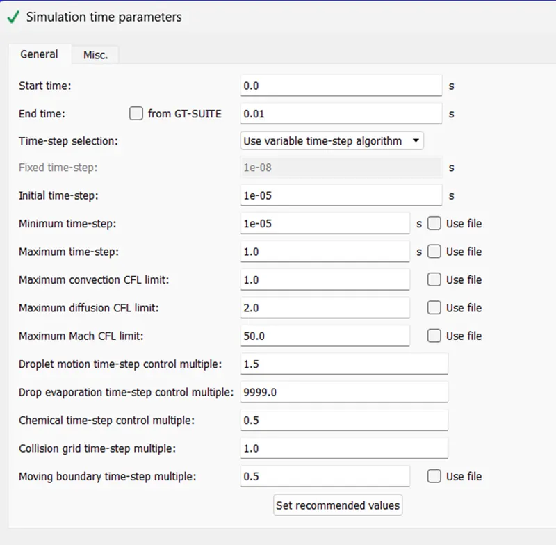
• Set up the Simulation Parameter as shown in the figure below.

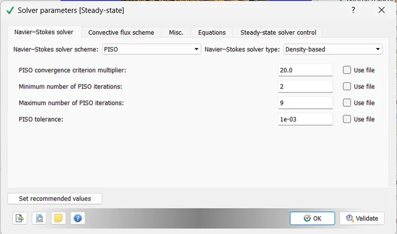
• For the Solver Parameter, select PISO for the solver scheme and Density-based solver type.
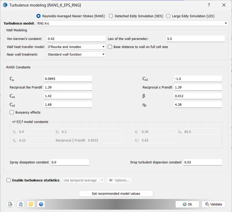
• For the Turbulence modelling, opt for RANS with the RNG k-epsilon model.
• In the Grid Control case setup, opt for Fixed Embedding.
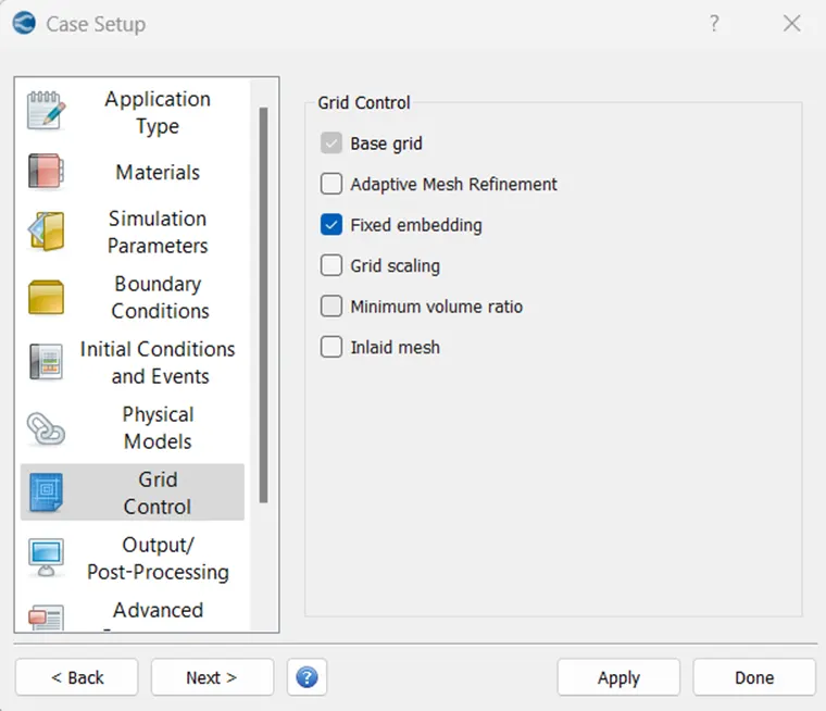
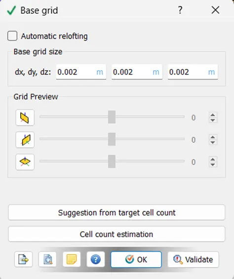
• Set the Base Grid size as 0.02m as shown in the below figure.
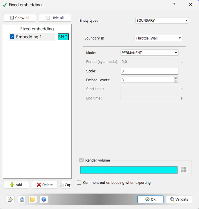
• Setup the embedding near the throttle wall with the scale of 3 and 3 embed layers to capture the boundary layer phenomenon near the throttle wall.

• Export the input file to the working folder.
• Open the working folder in the Cygwin terminal and run the simulation using the following command. ‘mpiexec.exe -n 4 converge.exe restricted </dev/null> logfile &’
• Post-process the results using ParaView.

Results:

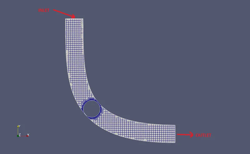
Mesh:

Pressure Plot

Static pressure Inlet vs Outlet

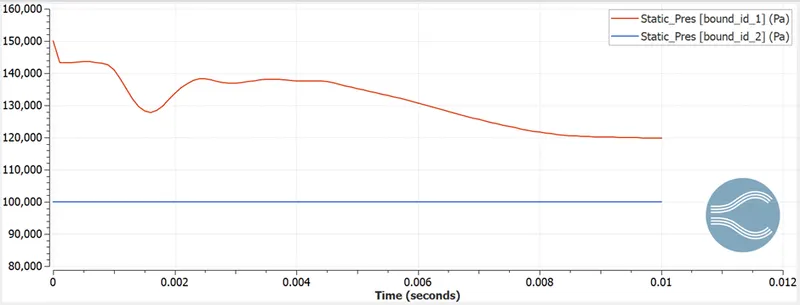
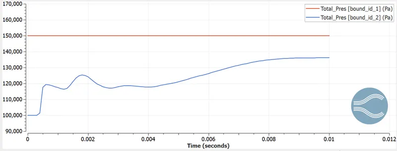
Total Pressure Inlet vs Outlet

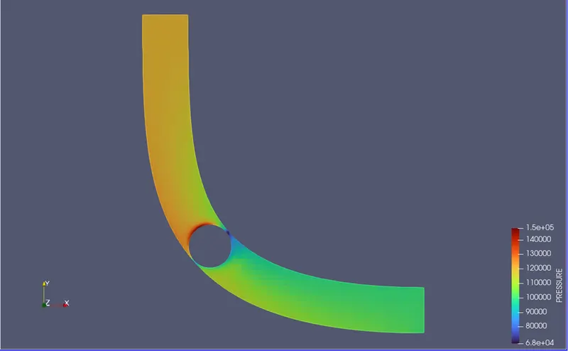
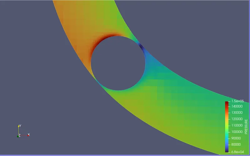
Pressure Contour

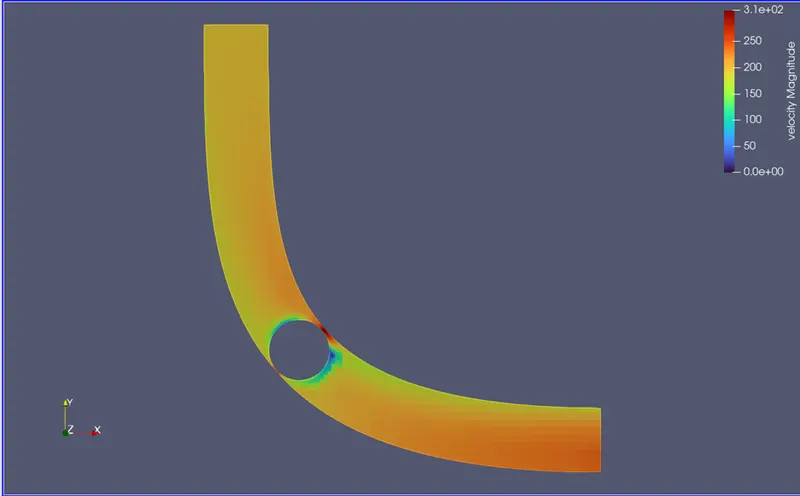
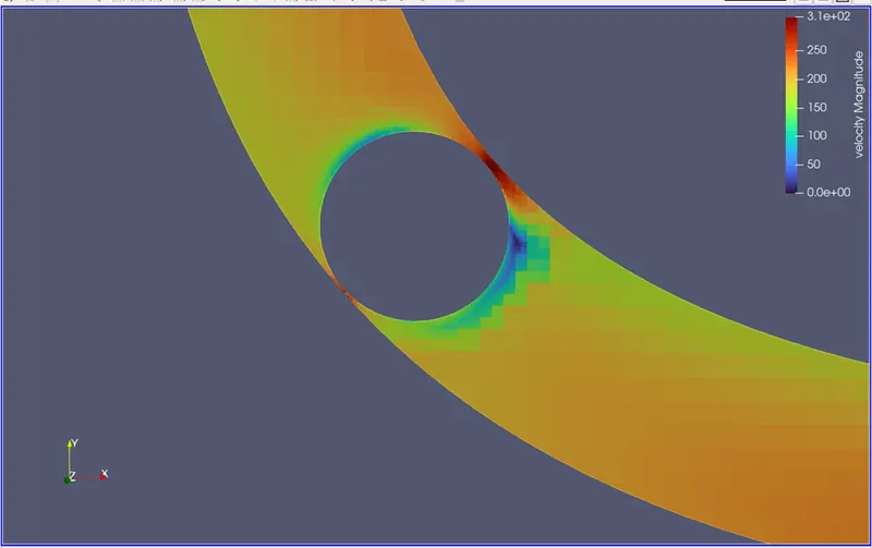
Velocity Plot

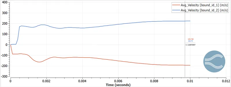
Average velocity Inlet vs Outlet

Velocity Contour

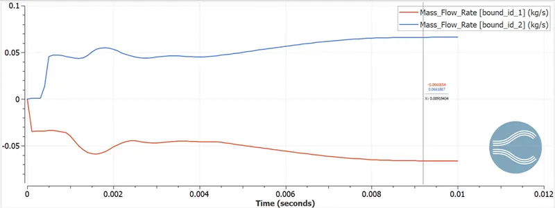
Mass Flow rate Plot

Mass flow rate Inlet vs Outlet

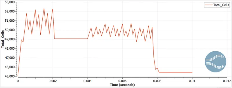
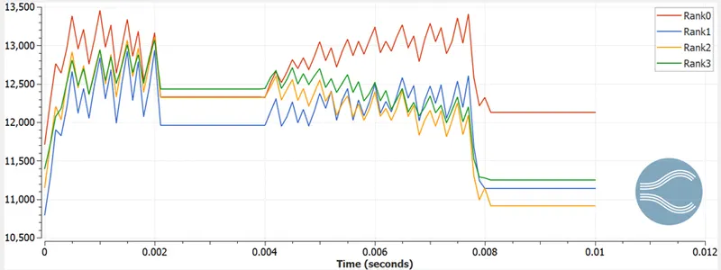
Total cell count

Cells allocated to different processors

Conclusion:

In this project, transient simulation on the throttle body is studied. Through contour plots for velocity and pressure, it is observed that the movement of the throttle affects the flow of the fluid in the elbow pipe.

The motion of the throttle can be observed in the video of contour plots.

Due to the moving boundary condition, the total cell count for the simulation change with respect to time.