Week 3.5 - Deriving 4th order approximation of a 2nd order derivative using Taylor Table method
Derivation for 4th order approximation of Second-order derivative using Taylor Table method
4th order approximation for a function can be obtained by using the following three schemes:
1. Central difference Scheme
2. Skewed right-sided difference Scheme
3. Skewed left-sided difference Scheme
Central Differencing Scheme
Since it is 4th order central scheme, the number of nodes required to write a hypothesis equation is determined using the thumb rule
The order of accuracy( P) = Number of nodes in the stencil (N) - order of derivative (Q ) + 1
4 = N - 2 + 1
N = 5
Then the hypothesis equation be

Each term is expanded using the Taylor series. Due to the complexity of writing and solving the equation, Taylor Table is introduced.
Taylor Table for the above equation is
| f (i).Δx0 | f'(i).Δx | f''(i).Δx2 | f'''(i).Δx3 | fiv (I) .Δx4 | |
| a. fi-2 | (-2)^0/0! = 1 | (-2)^1/1! | (-2)^2/2! | (-2)^3/3! | (-2)^4/4! |
| b.fi-1 | 1 | -1/1! | (-1)^2/2! | (-1)^3/3! | (-1)^4/4! |
| c.fi | 1 | 0 | 0 | 0 | 0 |
| d.fi+1 | 1 | 1/1! | (1)^2/2! | (1)^3/3! | (1)^4/4! |
| e.fi+2 | 1 | (2)^1/1! | (2)^2/2! | (2)^3/3! | (2)^4/4! |
| sum | 0 | 0 | 1 | 0 | 0 |
As we are about to find a second-order derivative, coefficients corresponding to f''(i) i.e derivative is assumed to be 1 and other than f''(i) as zero. And for 4th order approximation, we assume (O)Δx4 ≈0.
This table can be written in matrix form
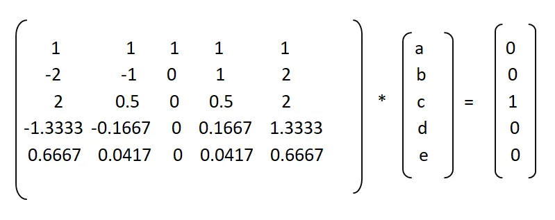
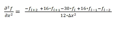
on solving above matrix using matrix inversion we get,
a= -1/12,
b= 16/12,
c =30/12,
d= 16/12,
e = -1/12,
Then,
Skewed Right side and Left side Approximation Scheme
Similarly, we can deduce the Skewed Right side and Left side Approximation Scheme using Taylor Table.
The number of nodes required to write the hypothesis equation is 6 derived from the thumb rule i.e. The order of accuracy P = Number of nodes in the stencil N - order of derivative Q.
The hypothesis equation for the Skewed Right side Scheme is

Also called as a 4th order Forward Differencing Scheme.
Taylor table for Skewed Right side Scheme
| f (i).Δx0 | f'(i).Δx | f''(i).Δx2 | f'''(i).Δx3 | fiv (I) .Δx4 | |
| a. fi | 1 | 0 | 0 | 0 | 0 |
| b.fi+1 | 1 | 1/1! | (1)^2/2! | (1)^3/3! | (1)^4/4! |
| c.fi+2 | 1 | (2)^1/1! | (2)^2/2! | (2)^3/3! | (2)^4/4! |
| d.fi+3 | 1 | 3/1! | (3)^2/2! | (3)^3/3! | (3)^4/4! |
| e.fi+4 | 1 | (4)^1/1! | (4)^2/2! | (4)^3/3! | (4)^4/4! |
| sum | 0 | 0 | 1 | 0 |
0 |
Matrix form
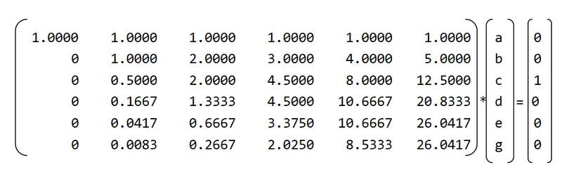
Using matrix inversion above simultaneous equation is solved.
we get,
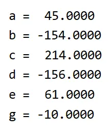
Then,

Skewed Left Side Scheme
And the hypothesis equation for the Skewed Left side Scheme is

Also called as a 4th order Backward Differencing Scheme.
Taylor table
| f (i).Δx0 | f'(i).Δx | f''(i).Δx2 | f'''(i).Δx3 | fiv (I) .Δx4 | |
| a. fi-4 | 1 | (-4)^1/1! | (-4)^2/2! | (-4)^3/3! | (-4)^4/4! |
| b.fi-3 | 1 | -3/1! | (-3)^2/2! | (-3)^3/3! | (-3)^4/4 |
| c.fi-2 | 1 | (-2)^1/1! | (-2)^2/2! | (-2)^3/3! | (-2)^4/4 |
| d.fi-1 | 1 | -1/1! | (-1)^2/2! | (-1)^3/3! | (-1)^4/4! |
| e.fi | 1 | 0 | 0 | 0 | 0 |
| sum | 0 | 0 | 1 | 0 | 0 |
Matrix form
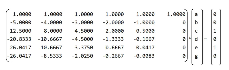
On solving the above simultaneous equation we get,
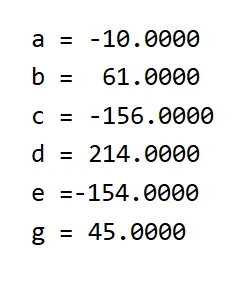
Then,

Main Program to Calculate Approximate Solution
close all
clear all
clc

x=pi/3;
dx=linspace(pi/4000,pi/40,20);
% Given function
f=cos(x)*exp(x);
% Terms

f1=cos(x+dx).*exp(x+dx); %f(i+1)
f2 =cos(x+2.*dx).*exp(x+2.*dx); %f(i+2)
f3 = cos(x+3.*dx).*exp(x+3.*dx); %f(i+3)
f4 = cos(x+4.*dx).*exp(x+4.*dx); %f(i+4)
f5 = cos(x+5.*dx).*exp(x+5.*dx); %f(i+5)

fa=cos(x-dx).*exp(x-dx); %f(i-1)
fb =cos(x-2.*dx).*exp(x-2.*dx); %f(i-2)
fc = cos(x-3.*dx).*exp(x-3.*dx); %f(i-3)
fd = cos(x-4.*dx).*exp(x-4.*dx); %f(i-4)
fe = cos(x-5.*dx).*exp(x-5.*dx); %f(i-5)
% Second order derivative of given function is f''= -2*sin(x)*exp(x)
% For Exact solution
exact=-2*sin(x)*exp(x);


for i=1:length(dx)

% Calculation of 4th order Approximation

% 4th Order Skewed Left Side Approximation Scheme/ Backward Differencing Scheme(FDS)
BDS(i)= (((-10.*fe(i))+(61.*fd(i))-(156.*fc(i))+(214.*fb(i))-(154.*fa(i))+45*f))./(12.*dx(i).^2);

% 4th Order Skewed Right Side Approximation Scheme/ Forward Differencing Scheme(BDS)
FDS(i)= (45*f-154.*f1(i)+214.*f2(i)-156.*f3(i)+61.*f4(i)-10.*f5(i))./(12.*dx(i).^2);

% 4th Order Central Approximation Scheme/ Cental Differencing Scheme(CDS)
CDS(i)=(-f2(i)+16.*f1(i)-30*f+16.*fa(i)-fb(i))./(12.*dx(i).^2);

% Error Calculation for different approximation solutions with exact solution
error_FDS(i) = abs(FDS(i)-exact);

error_BDS(i) = abs(BDS(i)-exact);

error_CDS(i) = abs(CDS(i)-exact);

end

% Plot
figure (1)
loglog(dx,error_FDS,'k')
hold on
loglog(dx,error_BDS,'r')
hold on
loglog(dx,error_CDS,'b')
hold off
xlabel('dx')
ylabel('Absolute Error')
title('Comparing Absolute Error for different schemes')
legend('FDS','BDS','CDS')
axis tight
%Slope Calculation

Slope_error_FDS= diff(error_FDS)/diff(dx)

Slope_error_BDS= diff(error_BDS)/diff(dx)

Slope_error_CDS= diff(error_CDS)/diff(dx)
Plot
Result
Conclusion
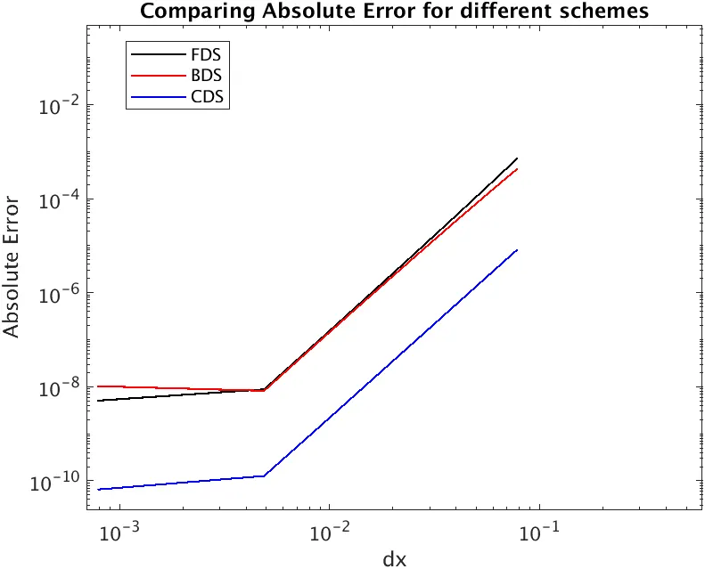
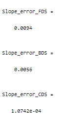
It is clear from the observation of plot and slope value of absolute error for the different schemes, the central differencing scheme is more approximate than the other two methods FDS and BDS.
Though CDS gives a more approximate solution than the other two, in most practical cases, the information flows in a single direction either forward or backwards. We cannot opt for CDS in such cases as we need information from all the neighbouring nodes.