Report on simulation of turbulent mixing of fluid flow inside Tee pipe

Aim and Objective

In this project, we are going to simulate the steady-state turbulent mixing of the hot fluid and cold fluid flow inside the Mixing Tee for 4 different cases.

Case 1

Short length Tee pipe with Momentum Ratio 2

Case 2

Short length Tee pipe with Momentum Ratio 4

Case 3

Long length Tee pipe with Momentum Ratio 2

Case 4

Long length Tee pipe with Momentum Ratio 4

The temperature of the hot fluid and cold fluid will be 36ᵒ C and 19ᵒ C respectively.

The momentum ratio is defined as the ratio of the fluid flow velocity at the cold inlet to the fluid flow velocity at the hot inlet.

Momentum Ratio = Velocity at cold inlet / Velocity at the hot inlet

The aim of the present project is as follows

• Simulating Steady State flow mixing inside Mixing Tees ( Short and Long ) using ANSYS Fluent
• Comparing the k-epsilon and k-omega SST models and choosing the suitable model for the current project.
• Perform a Mesh independent test for one of the cases.
• Plotting Velocity and Temperature contour plots on the cut planes along and across the pipe.
• Plotting Velocity and temperature line plots along and across the length of the pipe.
• Comparing Mixing Effectiveness for all the cases
• Comparing the Cell Count Value, Average Outlet Temperature, and Number of Iteration for Convergence for all the cases.
• Analyzing the effect of length and momentum ratio on the result of each case

The Objective of the project is to simulate, analyze and conclude the effect of the length of the Mixing Tee and the flow velocities of the fluids on the efficiency of the mixing of the two-fluid of different temperatures.

Theory

Mixing Tee

Mixing Tee is a pipe that is used to mix the two streams of fluids. In industries such as chemical, HVAC, etc. mixing tee is widely used to mix the fluids of different chemical compositions and physical properties, etc. into one stream together.

Hot fluid (Air) enters into the main pipe through the main inlet whereas the cold fluid (Air) entering from the tee and mixes inside the pipe. We are going to observe the effect of change in parameters like length of Mixing Tee, the velocity of the fluid flow, etc. on the temperature of the resultant fluid obtained at the outlet.

k-epsilon and k-omega turbulence models

k-epsilon and k-omega turbulence models are common types of models used in computation fluid dynamics to simulate turbulent flow.

k-epsilon turbulence model describes the turbulence through two transport equations with the help of two transport variables - turbulent kinetic energy (k) and rate of dissipation of turbulent kinetic energy (epsilon (ε)).

k-omega turbulence model is similar to the k-epsilon model which consists of two transport equations but the two transport variables are turbulent kinetic energy (k) and specific rate of dissipation (omega(ω)).

Procedure for Setup and run the simulation

The procedure for all the cases in this project will be the same as the below procedure.

Step 1: Setting the CAD Model (Pre-Processing)

1. Open ANSYS WORKBENCH and select the Fluid Flow (Fluent) in the Analysis System from the Toolbox and Double Click it or Drag it onto Project Schematic.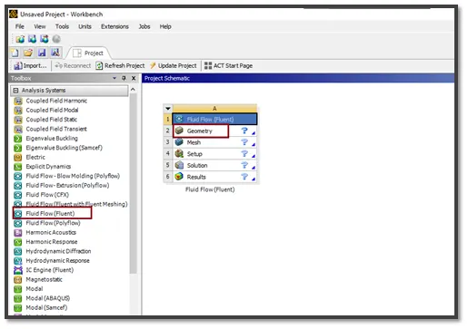

2. Double Click on Geometry to create the CAD model. It will open ANSYS Space Claim.

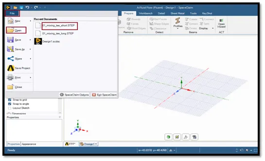
3. Since we already have the CAD model with we will import it into ANSYS Space Claim.

4. In ANSYS Space Claim, Click on File present in ribbon tools/menu click on OPEN. Find and select the CAD File. The Model is loaded.

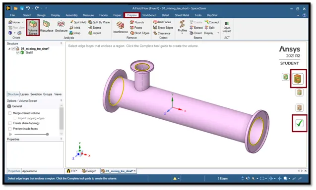
5. Since we are working on the volumetric part of the pipe we will extract the volume. Click on Prepare then on Volume Extraction. Click on Select Edges and select the edges as shown. Click on Right Symbol to extract volume.

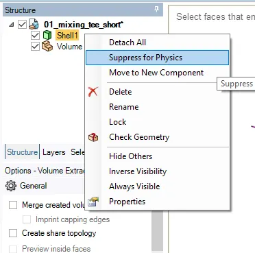
6. We aren’t going to use Pipe Wall surface for the analysis we will suppress the physics for the outer shell.

Right-click on shell in the left sidebar click on suppress the physics.

7. This is the required geometry for analysis.

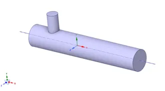
8. Close the Space Claim application.

Step 2: Meshing the Model (Pre-Processing)

1. Open Mesh by double-clicking it for meshing.

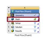
2. Give a label to the faces by Selecting the face and press ‘N’ and typing the name.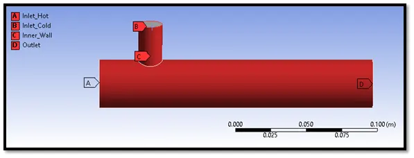

3. Since we creating a baseline mesh we will use default meshing. Click on Generate/ Update to generate the mesh.

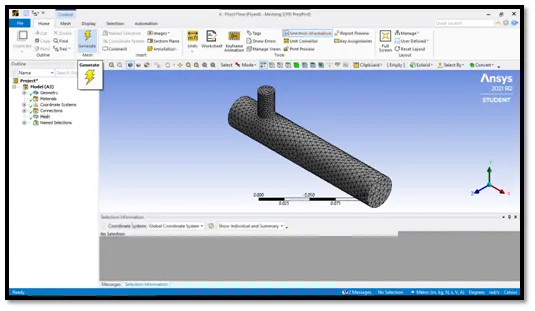
4. Check the element quality. Click on Mesh Display and Select Element Quality. Make sure that the element quality should not be less than 40%.

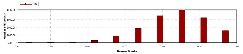
5. Close the Mesh. Update the mesh by right click on Mesh and Select Update.

Step 3: Setup the solver

1. Open ANSYS Fluent by double-clicking on Setup.

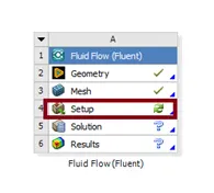
2. Click on Units in Domain and select Temperature to change the unit from Kelvin to Celsius. Click Close

3. Click Physics. Click the Energy Equation Check box as we are dealing with temperature heat change.

4. Click on Viscous Model present in models and Select k-omega model with SST. Click on OK and close it.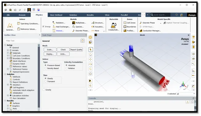

5. Boundary Conditions. To give boundary conditions click on boundaries present in the zone. In the Task Page, the dialog box selects the boundary which we want to set condition. Click on edit. A dialog box opens. In Momentum, Give velocity magnitude, and in Thermal give the temperature of the fluid.

6. Go to solution. We have to plot graphs of Area Weighted Average Temperature at Outlet wrt No. of Iteration and Standard Deviation of Temperature at outlet wrt to no. of iterations.

7. Initialize Solution. Since we will not give Boundary Condition at Outlet pressure we have to initialize the solution so that it can solve and have boundary conditions at the outlet. Click on initialization (as by default it is set to Hybrid Initialization) to initialize the solution.

8. Click on Run Calculation in Parameter section Set no. of iteration. Now hit on Calculate

9. After completion close Fluent. Update the solution by right click on fluent and Click on Update.

Step 4: CFD Post-Processing

In the Post Processing, we will be obtaining the result report of the simulation. In the following Result section, we will be discussing the results obtained from CFD Post.

Results

k-epsilon vs k-omega model

• To decide which model is most suitable for this project, we will be simulating a short mixing tee with a momentum ratio of 2.
• The models we are using for this case are k-epsilon Realizable and k-omega SST

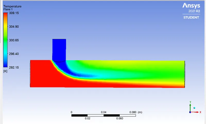
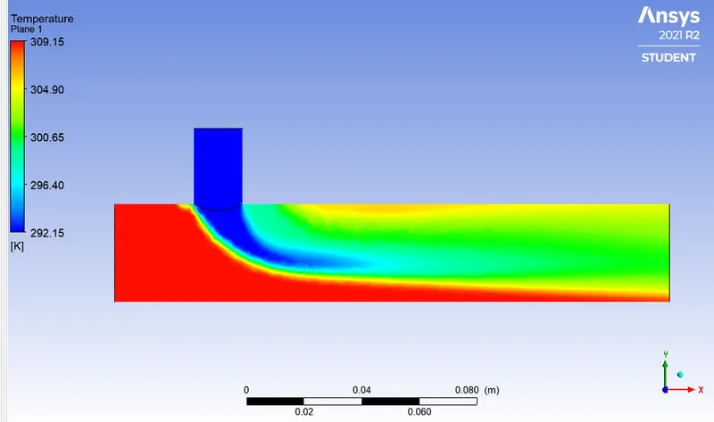
Fig 1. Temperature contour for (a) k-epsilon model (b) k-omega model

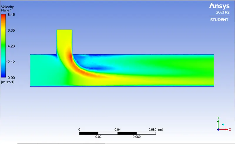
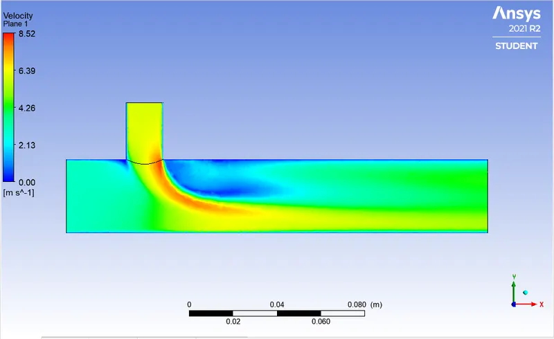
Fig 2. Velocity contour for (a) k-epsilon model (b) k-omega model

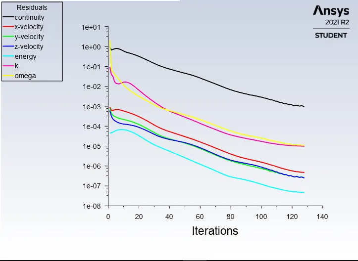
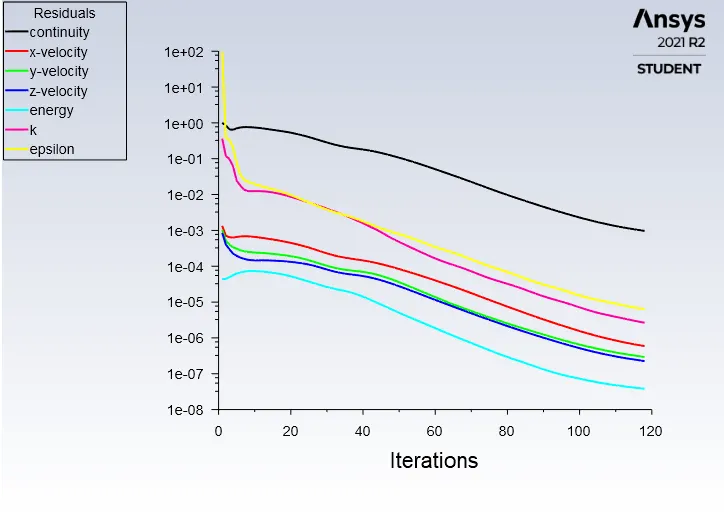
Fig 3. Convergence plot for (a) k-epsilon model (b) k-omega model

Observations from the above results

• The average temperature of the fluid mixture at the outlet for the k-epsilon is 30.399 C and for the k-omega model, it is 30.461 C, which is nearly equal.
• If we observe the temperature and velocity contour, the k-omega model predicts turbulence near the wall more accurately than the k-epsilon model.
• Number of iterations for convergence of solution from the k-omega model is more than the k-epsilon model. K-omega model takes more time for the solution than k-epsilon.
• Since we are simulating a small-scale problem, we choose the k-omega SST model over k-epsilon Realizable model. Though the k-omega SST model takes more iterations it gives more accurate results.

Mesh Independence Test

• Mesh independent test is taken to determine the dependency of the results with the mesh resolution or mesh density.
• By thumb rule, we know that accuracy of a solution increases with the increase in the number of mesh elements. But after a certain limit, there will be no significant change in solution on further refinement of mesh.
• It is important to check for mesh independence as it helps to find a minimum number of mesh elements required for optimum solution time.
• Initially, we began with the coarse mesh and we refine it further. On every step, we will be noting down the results in order to observe the change in the solution with respect to the mesh refinement.
• We performed a mesh independence test on case 1: short mixing tee with a momentum ratio of 2 and the following are the data obtained.

No. of Elements	Outlet Temperature
12403	30.258
14051	30.257
60659	30.381
330442	30.426

Results from Simulation for

1. Short Mixing Tee with momentum ratio 2

Convergence Plots

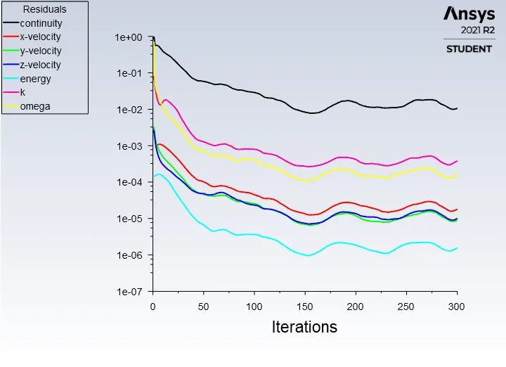
Fig. Convergence plot for Residuals of governing and transport equations

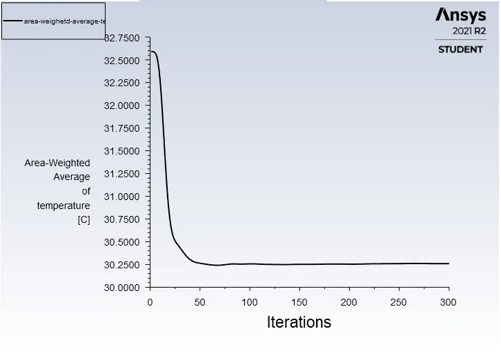
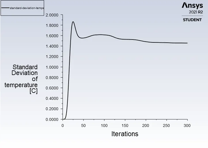
Fig. Area Weighted Average and Standard Deviation of outlet temperature

Temperature Contour Plot

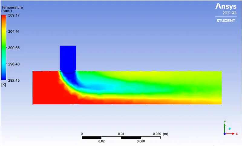
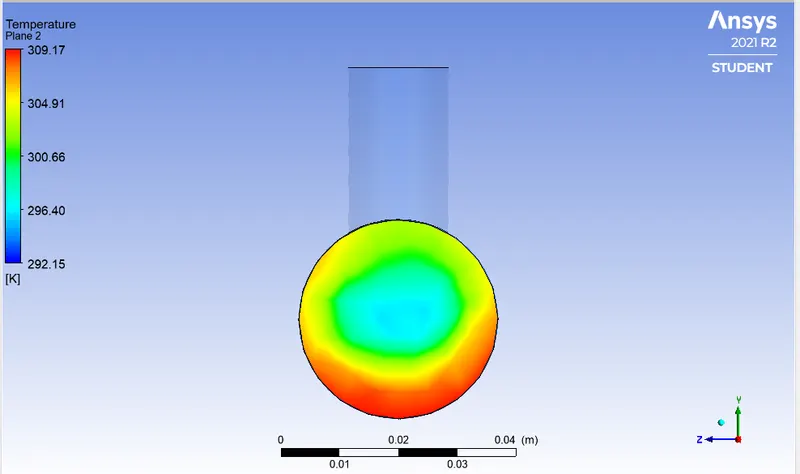
Fig. Temperature Contour on the plane (a) Along and (b) Across the pipe

Velocity Contour Plot

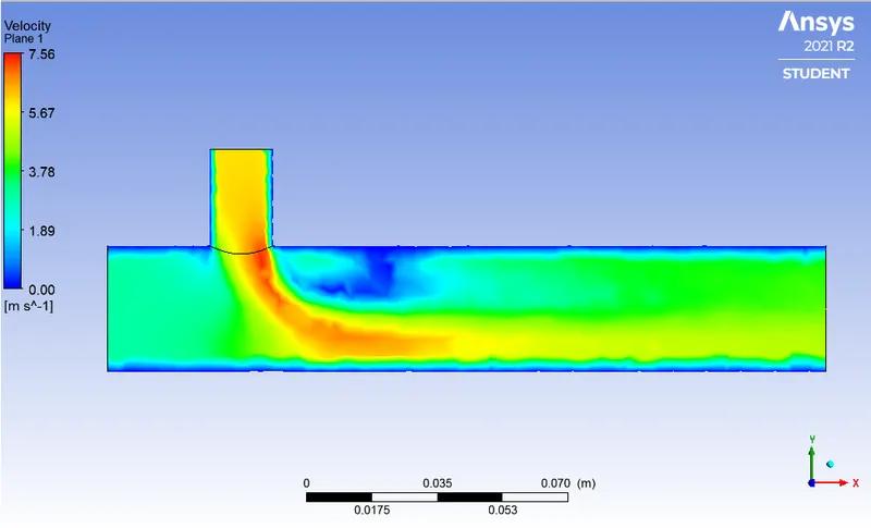
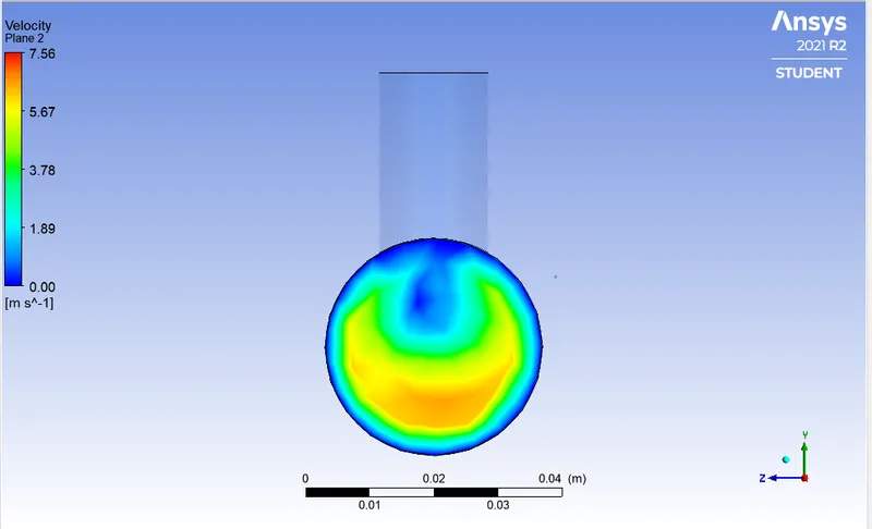
Fig. Velocity Contour on the plane (a) Along and (b) Across the pipe

Temperature Line Plot

For plotting the Temperature and Velocity line plot, temperature and velocity values along the lines, drawn on the planes as shown in the below diagram, are taken.

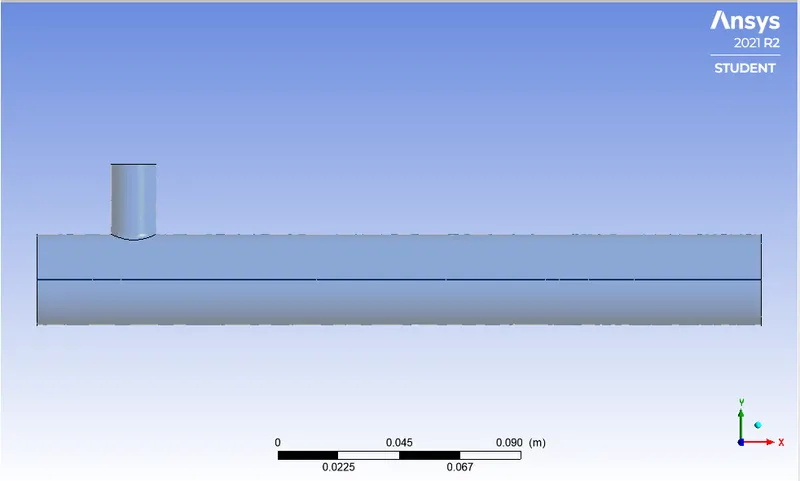
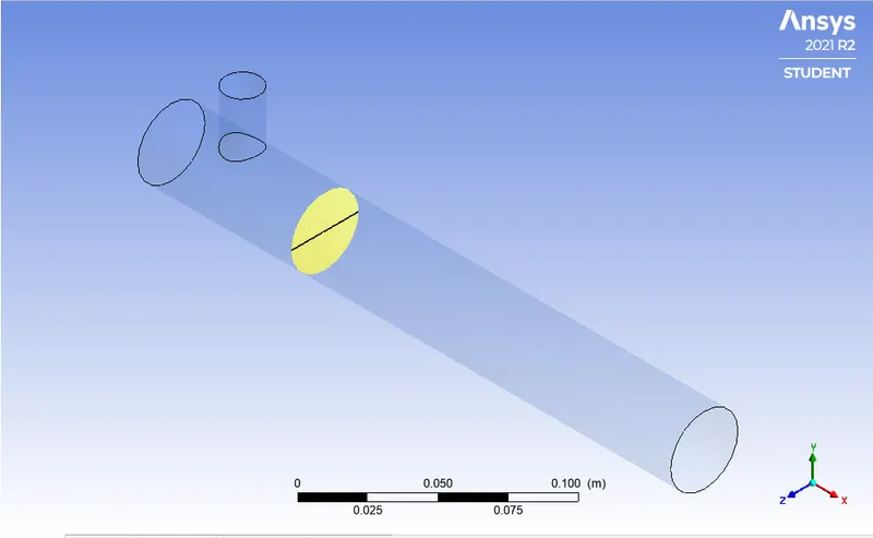
Fig. Line drawn along and across the pipe

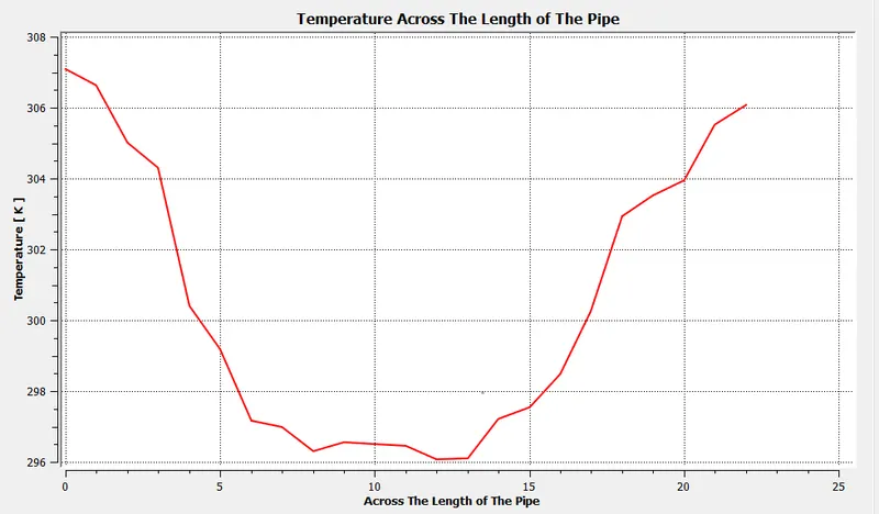
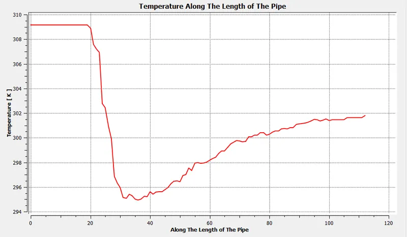
Fig. Line Plot for Temperature (a) Across and (b) Along the Pipe

Velocity Line Plot

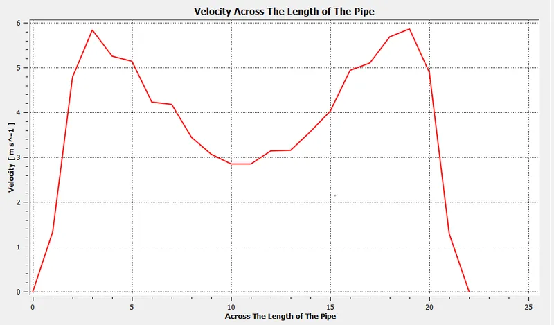
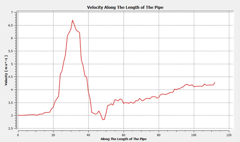
Fig. Line Plot for Velocity (a) Across and (b) Along the Pipe

2. Short Mixing Tee with momentum ratio 4

Convergence Plots

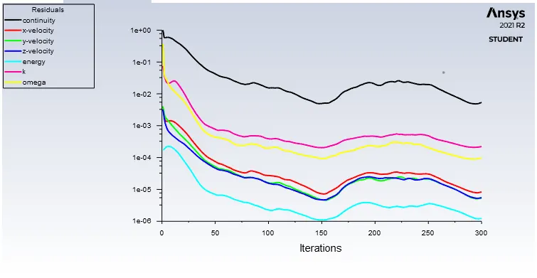
Fig. Convergence plot for Residuals of governing and transport equations

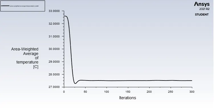
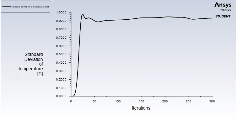
Fig. Area Weighted Average and Standard Deviation of outlet temperature

Temperature Contour Plots

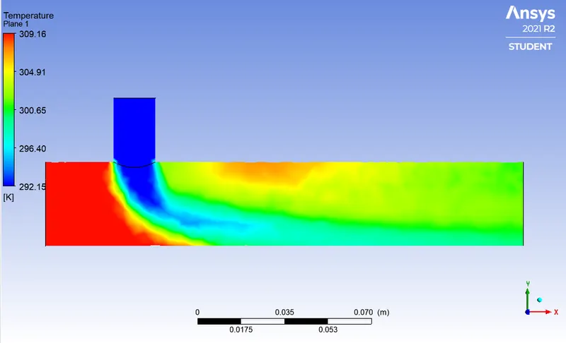
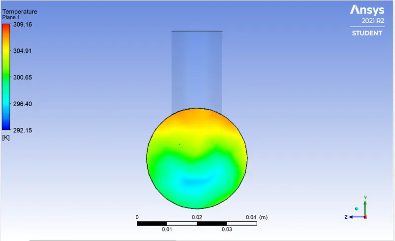
Fig. Temperature Contour on the plane (a) Along and (b) Across the pipe

Velocity Contour Plots

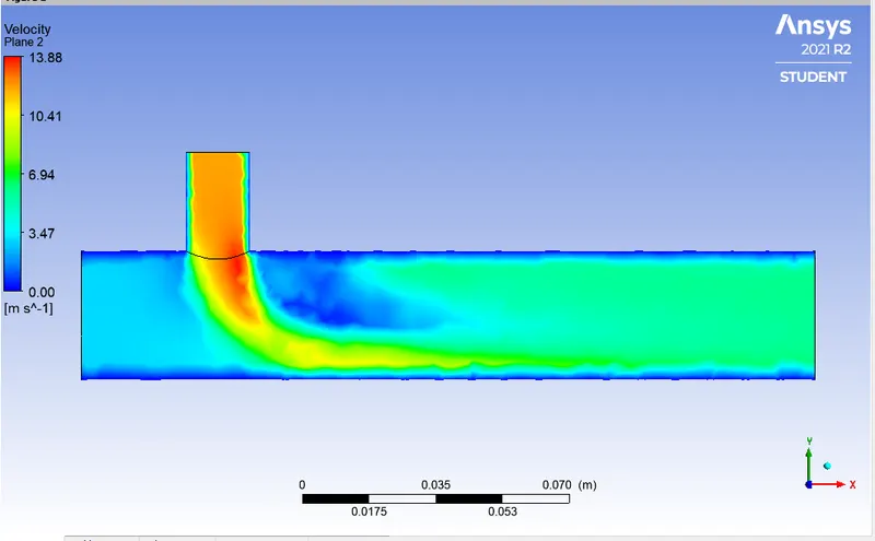
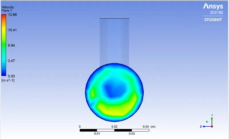
Fig. Velocity Contour on the plane (a) Along and (b) Across the pipe

Temperature Line Plots

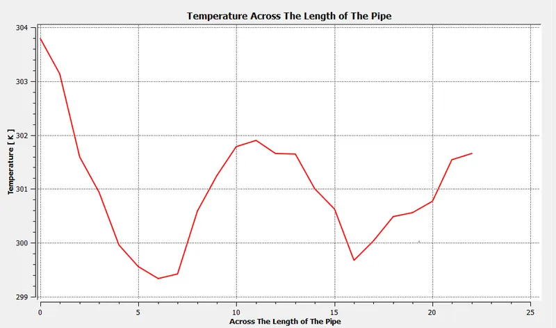
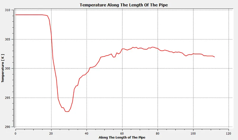
Fig. Line Plot for Temperature (a) Across and (b) Along the Pipe

Velocity Line Plots

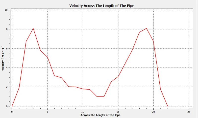
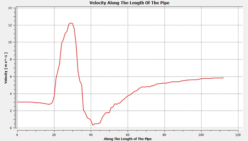
Fig. Line Plot for Velocity (a) Across and (b) Along the Pipe

3. Long Mixing Tee with momentum ratio 2

Convergence Plots

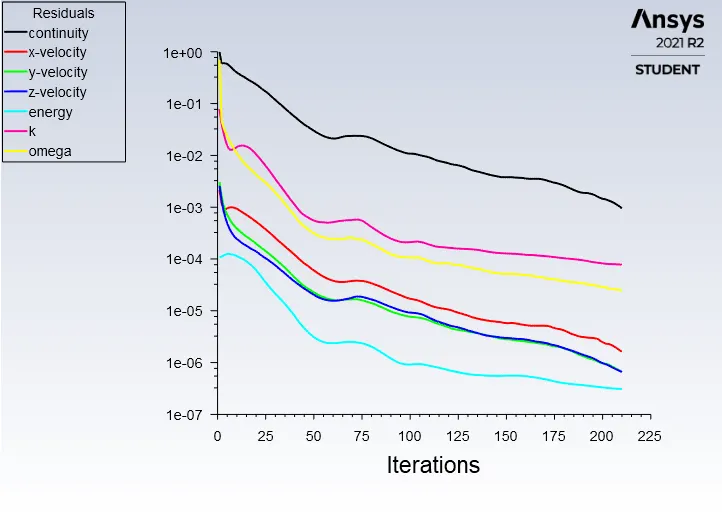
Fig. Convergence plot for Residuals of governing and transport equations

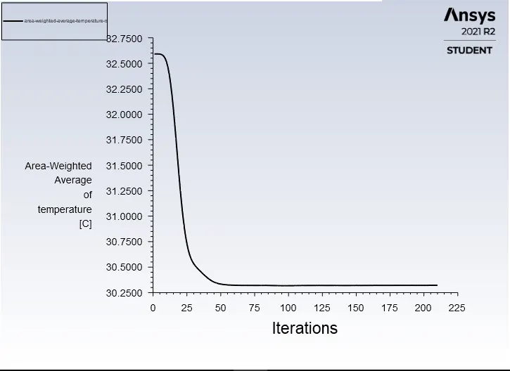
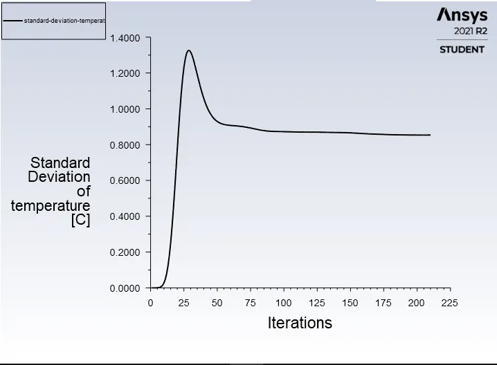
Fig. Area Weighted Average and Standard Deviation of outlet temperature

Temperature Contour Plots

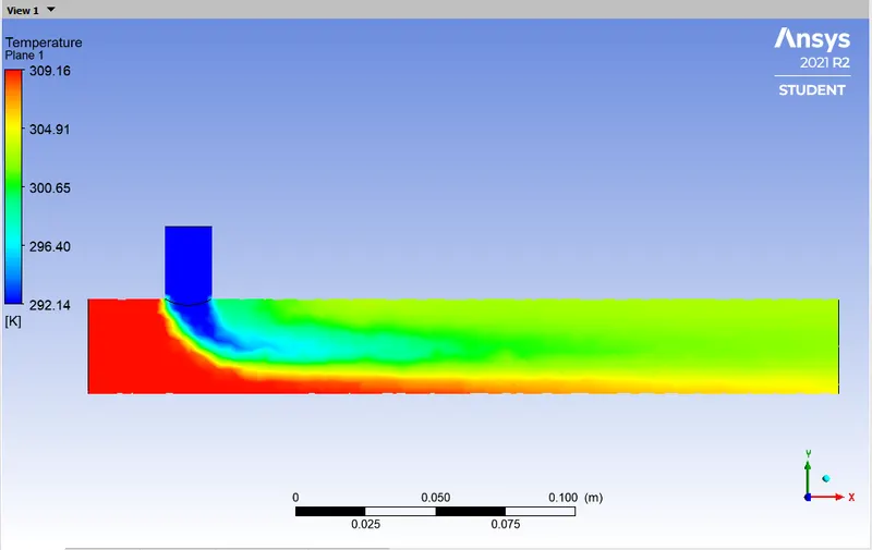
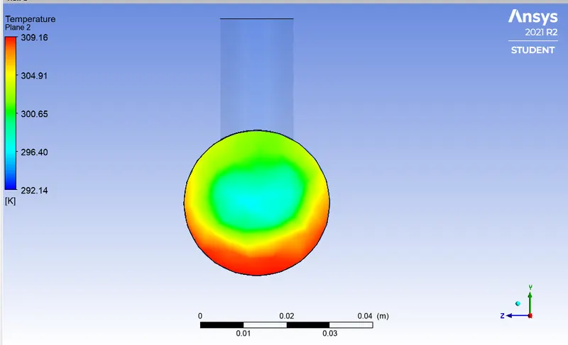
Fig. Temperature Contour on the plane (a) Along and (b) Across the pipe

Velocity Contour Plots

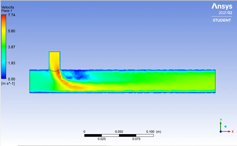
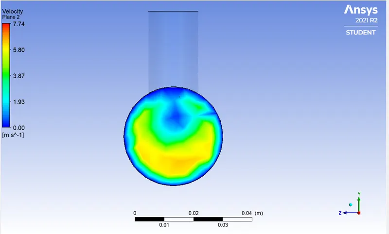
Fig. Velocity Contour on the plane (a) Along and (b) Across the pipe

Temperature Line Plots

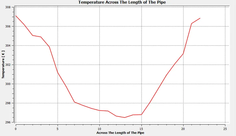
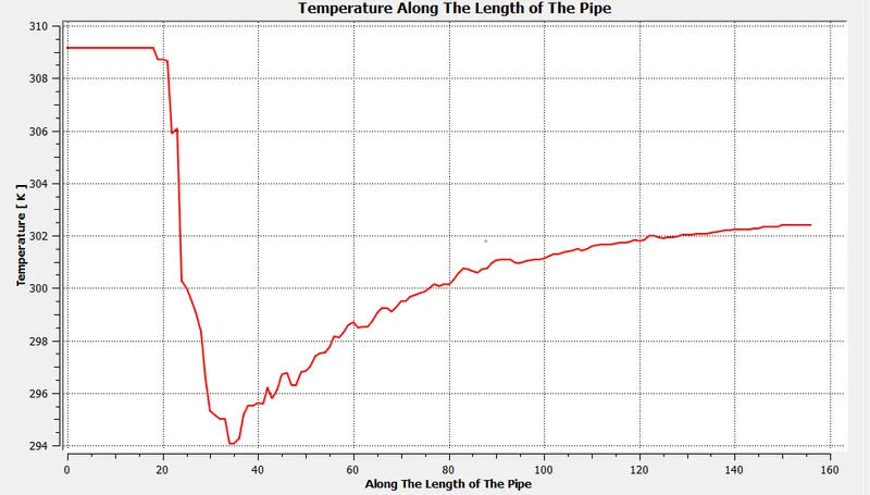
Fig. Line Plot for Temperature (a) Across and (b) Along the Pipe

Velocity Line Plots

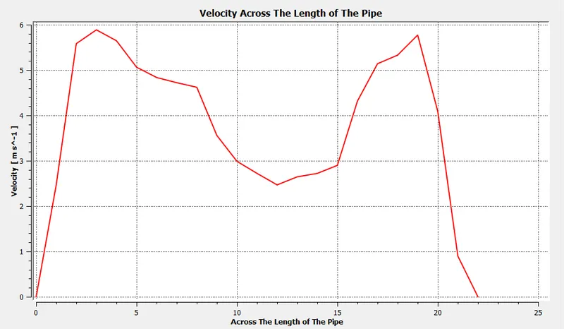
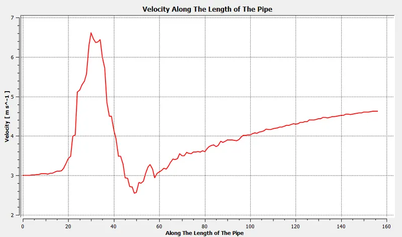
Fig. Line Plot for Velocity (a) Across and (b) Along the Pipe

4. Long Mixing Tee with momentum ratio 4

Convergence Plots

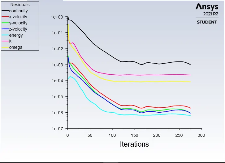
Fig. Convergence plot for Residuals of governing and transport equations

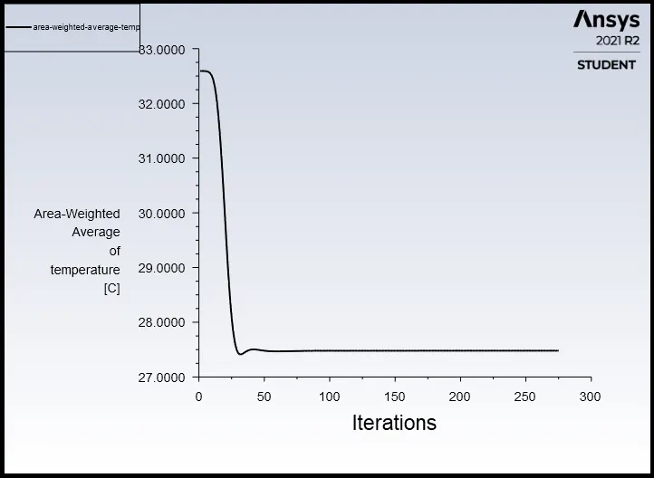
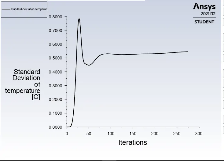
Fig. Area Weighted Average and Standard Deviation of outlet temperature

Temperature Contour Plots

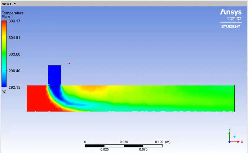
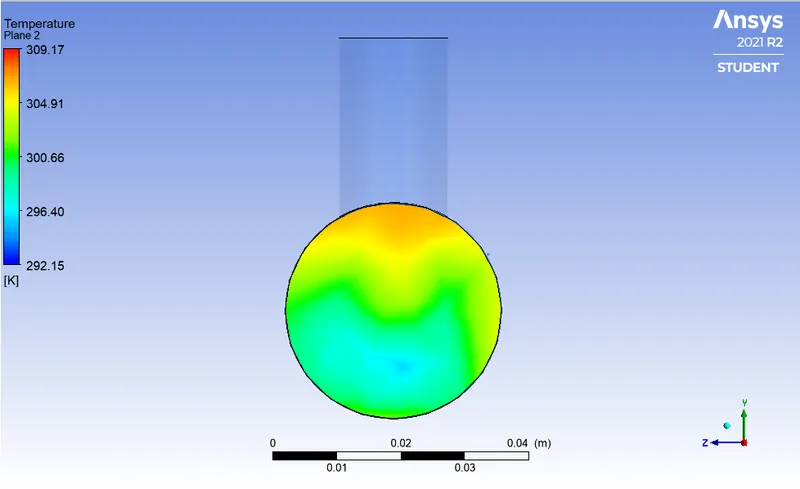
Fig. Temperature Contour on the plane (a) Along and (b) Across the pipe

Velocity Contour Plots

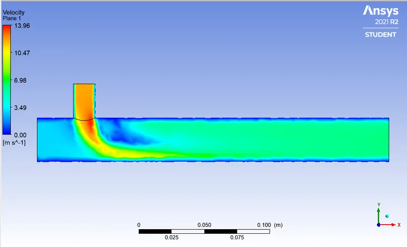
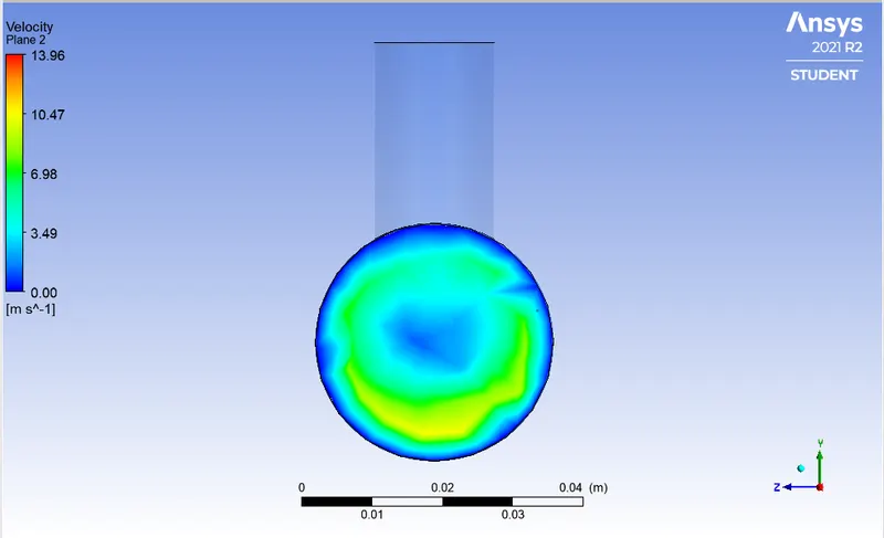
Fig. Velocity Contour on the plane (a) Along and (b) Across the pipe

Temperature Line Plots

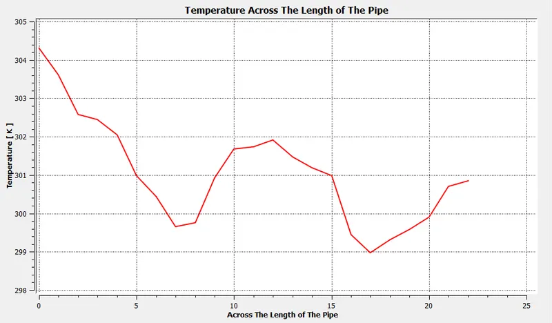
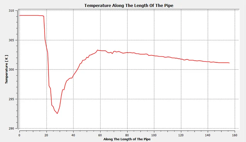
Fig. Line Plot for Temperature (a) Across and (b) Along the Pipe

Velocity Line Plots

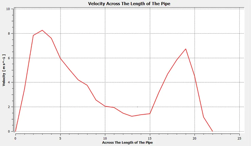
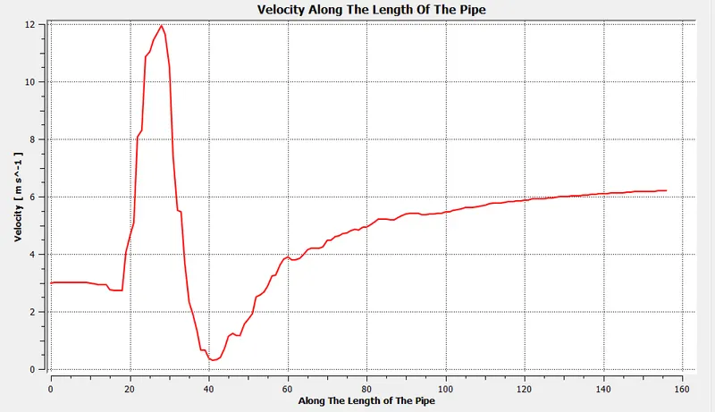
Fig. Line Plot for Velocity (a) Across and (b) Along the Pipe

Analytical Solution

The analytical Temperature of the mixture at the outlet is be calculated using the formula below

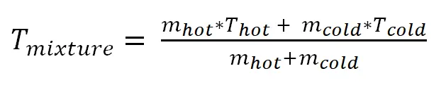
Since mass flow rate `m = rho*A*V`

then `m_(hot) = rho_(air)**A_(hot)**V_(hot)=1.225**0.0089779**3`

`m_(hot)=0.003299`kg/s

for momentum ratio of 2 `m_(cold) = rho_(air) **A_(cold)**V_(cold) = 1.225**0.00022484**6`

`m_(cold) = 0.0016625`kg/s

and the temperature of the mixture for momentum ratio 2 is`T_(mixture) = 30.326^o C`

for momentum ratio of 4

`m_(cold) = rho_(air)**A_(cold)**V_(cold) = 1.225**0.00022484**12`

`m_(cold) = 0.0033051`kg/s

and the temperature of the mixture for momentum ratio 4 is `T_(mixture) = 27.492^o C`

The following table compares the analytical results with the simulation results

Momentum Ratio	Analytical	Short	Long
2	30.326 C	30.26 C	30.32
4	27.492	27.51	27.48

It is observed that prediction from the simulation is much accurate with an error > 0.1%

Conclusions

• Though the simulation time taken for solving the k-omega SST model is more than k-epsilon Realizable model, the k-omega SST model gives a more accurate prediction of turbulence.
• Comparison table

  Case	Cell Count	Avg. Outlet Temperature	No. of Iteration for Convergence
  Short with mr 2	12403	30.26	228
  Short with mr 4	12403	27.51	304
  Long with mr 2	15429	30.32	210
  Long with mr 4	15429	27.48	275

mr is momentum ratio

• We observed from the data that the length of the mixing tee doesn't bring any significant change in the fluid mixture temperature. Whereas the increase in momentum ratio leads to a decrease in outlet fluid mixture temperature.
• Among all 4 cases, we conclude that a Long mixing tee with a momentum ratio of 4 is the most efficient in mixing the fluid. Change in momentum ratio brings a very significant change in mixture temperature whereas the length of the pipe becomes insignificant.
• The mixing efficiency of the mixture mostly depends on the momentum ratio.