Week 9 - FVM Literature Review
LITERATURE REVIEW ON FINITE VOLUME METHOD
In computational fluid dynamics, problems are solved using numerical analysis and numerical methods. Following are the numerical methods use for discretization
- Finite Difference Method
- Finite Volume Method
- Finite Element Method
Finite difference method
Finite difference method is a numerical method that involves solving the differential equation by approximating the derivatives. The fundamental continuum equation is in the form of a partial differential equation that is discretized using Taylor series expansion and converted into a set of linear algebraic equations also known as a finite difference equation.
The most advantageous feature of FDM is its simplicity as we can write a finite difference equation for any differential equation without much manipulation using Taylor series expansion
But there is a drawback regarding the geometry. In the case of complex curvilinear geometry, it is required to convert the geometry from the cartesian coordinate system to the local coordinate system with the help of mapping function and solving the problem and then again converting the equation into cartesian form to obtain the actual solution. This process makes the Finite Difference Method laborious and complicated to implement for such geometries.
Also, a fundamental problem arises due to the truncation of the Taylor series by neglecting the higher-order terms in the series, leading to a rise of a significant error in the overall solution.
Another drawback in Taylor series expansion-based discretization is that the absence of conservativeness. If a physical problem involves the conservation of a dependent variable, let's say conservation of mass or momentum, then the summing of the discrete equations over the entire domain should also represent the same principle of conservation that is observed in the physical problem. In FDM, we can observe a lack of conservativeness as in the fundamental process of discretization in FDM, conservation of equation is never enforced.
Finite volume method
In the finite volume method, the whole domain is divided/discretized into non-overlapping finite-size subdomains also known as control volume. Then the governing differential equation is converted into integral form by integrated over the control volume and converted into to surface integral using Gauss-diversion theorem.
Need of interpolation function
With the help of interpolation or approximation function, the surface integral form is converted into a set of algebraic equations. These algebraic equations represent the function of the dependent variable at corresponding grid points (in this case, centroid of control volume ) similar to the finite difference method. Following are some of the interpolation schemes
- Upwind scheme
- Linear interpolation
- QUICK - Quadratic upwind interpolation scheme
- Hybrid scheme.
Since surface integrals are evaluated on the surface of control volume which is obtained by discretizing the entire domain, the flux that entering and leaving the control volume is conserved. This feature of FVM makes it suitable and applicable for problems based on fluid flow and heat transfer where dependent variables are needed to be conserved.
Need for flux limiter in FVM
Flux limiters are limited values that limit the gradient value when there is
- High gradient value
- Discontinuities
- functions that are similar to boundary conditions.
Flux limiter plays an important role to limit the spatial derivative while solving partial differential equations for higher resolution schemes.
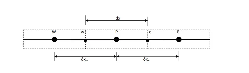
The finite volume method can be better understood with the following example.
Consider a 1D steady-state heat conduction without heat generation
`d/(d x) (k (d T)/(d x)) = 0`
where k is linear thermal diffusivity,